2D Kinematics and Dynamics
Tl;DR
A summary of 2D mechanics for multibody systems.
Intro
I vibecoded in one shot a static cool page about multibody: https://multibodysystemdynamics.pages.dev/
And ended up taking back mbsd where I left it during spring of 2023.
How much things have changed since then…
I mean, same physics.
But…
Lets say that now migration from Matlab to Python is waaay faster.
About MBSD
Code is law, specially for multibody system dynamics.
git clone git clone https://github.com/JAlcocerT/mbsd
This is obviously superseeding:
Kinematics
With just kinematics and the learnings inside the 3D-Design repository…
You can do cool stuff already.
cd ./3D-Design/mbsd-to-render/bicycle_leg
#make help
Once rendered at my x300, I bring it to my x13 via rsync:
make all
rsync -avP jalcocert@192.168.1.2:/home/jalcocert/3Design/mbsd-to-render/bicycle-leg/render/bicycle_leg.mp4 .
mpv bicycle_leg.mp4
This is the flow:
flowchart LR
    A[q₀ initial guess] --> B[Position solve:
C q,t = 0
Newton-Raphson]
    B --> C[Velocity solve:
Cq·v = -Ct]
    C --> D[Acceleration solve:
Cq·a = -DCq·v + Ctt]
    D --> E[Store q, v, a at tᵢ]
    E --> F{Next t?}
    F -->|yes, q₀ := q| B
    F -->|no| G[Done]
Implemented 2D Constrains
A holonomic constraint is an equation of the form C(q, t) = 0 that
must hold at every time.
“Holonomic” means it depends only on positions (and possibly explicit time), not on velocities.
All the joints in this series are holonomic.
Common 2D joint types and the number of equations each contributes:
| Joint | Geometric meaning | Equations |
|---|---|---|
| Revolute (pin) | Two body-fixed points coincide in world | 2 |
| Prismatic (slider) | Same angle + one point stays on a fixed line | 2 |
| Point-on-line | One body-fixed point stays on a line defined by another body | 1 |
| Cam/Leva | Two parameterised surfaces stay in tangent contact | 3 (+ 2 extra coords per joint) |
| Gear | θ_i − τ·θ_j = 0 (fixed transmission ratio) | 1 |
| User | Any scalar equation C_user(q, t) = 0 (driving motion, locks, …) | 1 or more |
Plus three equations pinning the ground body at x_0 = y_0 = θ_0 = 0.
Stacking all constraint equations gives the constraint vector C(q, t) ∈ ℝ^{n_restr}. The system’s physical degrees of freedom are
n_DOF = n_coord − n_restrFor a slider-crank driven by a user constraint that prescribes the crank
angle, n_DOF = 0 — the mechanism’s motion is completely determined.
Without that user constraint,
n_DOF = 1— the crank can spin freely.
Dynamics
Understand constrained dynamics and how to simulate real mechanisms with 2D motions.
cd ./mbsd/2D-DynamicsVideo Sequence in _all.mp4
The combined video now shows the complete causality chain:
- Forces (gravity + applied torque)
- Constraints (gravity vs constraint forces) ← NEW!
- Accelerations (F = ma)
- Velocities (∫a dt)
- Energy Flow (validation)
See a diagram of the dynamics flow
Physics x Lagrangian
The Physics: Constrained Lagrangian Mechanics
M·a = Q_total = Q_gravity + Q_constraint + Q_applied
The Equation We Solve
M(q) @ a + ∇V(q) = Q_ext + C_q^T @ λWhere:
- M(q) = Mass matrix (constant in reference coordinates)
- a = Acceleration vector (what we compute)
- ∇V(q) = Potential energy gradient (gravity effects)
- Q_ext = External forces (torques, springs, user input)
- C_q^T @ λ = Constraint reaction forces (the hidden part!)
- λ = Lagrange multipliers (automatic, varies with config)
The Constraint Equations
C(q, t) = 0              ← Joint constraint (position)
C_q @ v = ∂C/∂t          ← Velocity constraint (automatic)
C_q @ a = -dC_q @ v - d²C/dt²   ← Acceleration constraint
The Mathematical Recipe for 2D Dynamics
This is a high-level summary of the mathematical “recipe” used to solve the dynamics
To move from a static description of a mechanism to a living simulation, we follow a four-step mathematical process rooted in Lagrangian Mechanics.
- Define the System State
We represent every rigid body $i$ using three coordinates: $q_i = [x, y, \theta]^T$.
For a system of $n$ bodies, the global state vector is:
$$q = [q_1, q_2, \dots, q_n]^T$$
- Apply Geometric Constraints
Physical joints (pins, sliders, gears) are represented as algebraic equations that must equal zero:
$$C(q, t) = 0$$
To solve for motion, we must know how these constraints change as the bodies move.
We find the Jacobian ($C_q$) by taking the partial derivative of the constraints with respect to the coordinates:
$$C_q = \frac{\partial C}{\partial q}$$
- Assemble the Equations of Motion
Using the Principle of Virtual Work and the Lagrange Multiplier method, we combine Newton’s second law ($F = ma$) with our constraints.
This results in the Saddle-Point System:
$$\begin{bmatrix} M(q) & C_q^T \ C_q & 0 \end{bmatrix} \begin{bmatrix} a \ \lambda \end{bmatrix} = \begin{bmatrix} Q_{total} \ \gamma \end{bmatrix}$$
- $M(q)$: The mass and inertia of all bodies.
- $a$: The unknown accelerations we want to find.
- $\lambda$: The unknown Lagrange Multipliers (the reaction forces at the joints).
- $Q_{total}$: External forces like gravity, springs, and motor torques.
- $\gamma$: The “acceleration RHS,” which handles the inertial effects of the constraints ($C_q \cdot a = \gamma$).
- Integrate or Extract
Depending on the goal, we use the results of that matrix solve in two ways:
- Forward Dynamics: We take the accelerations ($a$), add them to the current velocities, and update the positions using a time-integrator (like Runge-Kutta). This “plays” the simulation forward.
- Inverse Dynamics: If the motion is already prescribed (e.g., we know the crank must spin at 10 RPM), we solve for $\lambda$ to find out exactly how much torque the motor needs to provide and how much stress the bearings are under.
By repeating this solve hundreds of times per second, we capture the high-frequency vibrations and inertial “shakes” characteristic of complex mechanical systems.
2D Direct Mechanics
Given certain forces - where does the mbsd position evolve over time?
2D Inverse Mechanics
Given a defined trajectory - what are the forces that make it possible?
Thats not a problem, see this script for a slider crank rotating at constant speed.
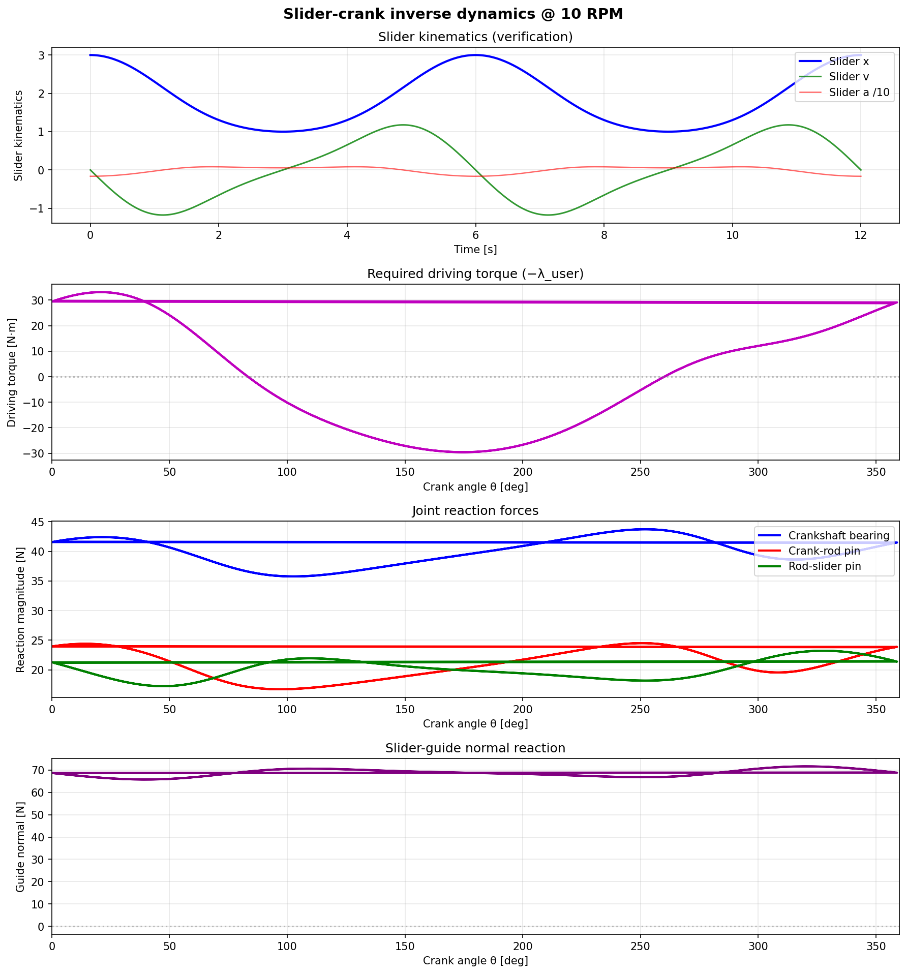
Given a kinematically-driven trajectory (mechanism with DOF = 0 thanks to
user constraints), compute the Lagrange multipliers = constraint reaction
forces at every time step.
No integration — just a kinematic sweep plus the saddle-point solve.
The classic ME use case: “I need my crankshaft to rotate at 10 RPM — what driving torque do I supply, and what loads do the bearings see through the cycle?”
A 2D MBSD Simulator
As Im preparing for 3D, just thought that matplotlib could be insufficient.
I got to know about 3JS: https://threejs.org/
Just tweaked the architecture and made it hybrid…
#git clone https://github.com/JAlcocerT/mbsd
cd /home/jalcocert/Desktop/mbsd/2D-Dynamics && source venv/bin/activate && python3 examples/export_for_viewer.py
#cp /home/jalcocert/Desktop/mbsd/2D-Dynamics/viewer/data/slider-crank*.json /home/jalcocert/Desktop/mbsd/2D-Simulator/viewer/data/ && ls -lh /home/jalcocert/Desktop/mbsd/2D-Simulator/viewer/data/*.json
That will generate a JSON export with what the mechanism do.
Meaning snapshots of its position defined overtime
To visualize whats coming: and debug
#cd ./mbsd/2D-Dynamics

cd /home/jalcocert/Desktop/mbsd/2D-Simulator
python3 visualize_json.py viewer/data/slider-crank-no-gravity.json --frame 0 --output reference_frame_0.png

# Visualize frame 0 (initial position)
python3 visualize_json.py viewer/data/slider-crank-no-gravity.json

# Visualize a specific frame and save as PNG
python3 visualize_json.py viewer/data/slider-crank-no-gravity.json --frame 50 --output frame_50.png

# Works with any mechanism JSON
python3 visualize_json.py viewer/data/slider-crank.json --frame 100 --output gravity_frame.png
Now to visualize it: thanks to threeJS, we have some kind of augmented reality :)
cd ./mbsd/2D-Simulator
npm install
This installs:
- Three.js - 3D WebGL rendering library
- Vite - Fast development server
- dat.gui - UI controls (for future enhancements)
npm run devWe already capture all this data in the JSON:
trajectory_data = {
    "time": [float(t) for t in t_dyn],
    "positions": [...],
    "velocities": [...],        # ← Already have this
    "accelerations": [...],     # ← Already have this
    "tau_applied": [...],       # ← Constraint forces at joints
    "energy": {                 # ← Already computing
        "kinetic": [...],
        "potential": [...],
        "total": [...]
    }
}
What we could visualize (Phase 2):
- Velocity vectors — arrows at joints showing speed magnitude/direction
- Acceleration vectors — arrows showing acceleration at points
- Force vectors — arrows at constraint points showing internal forces
- Color-coded bars — bars colored by velocity/acceleration magnitude
- Energy flow — animate kinetic↔potential energy transfers
- Vector trails — show historical path of joint motion
Conclusions
A mechanism is an MBody object with:
| Attribute | Contents |
|---|---|
bodies | list of Body(name, mass, inertia, rG); body 0 is always ground |
rev_joints | list of RevJoint(i, j, ri, rj) — revolute pair between body i and j at local points ri, rj |
prism_joints | PrismJoint(i, j, ri, rj, hi) — prismatic, hi defines sliding direction normal |
punto_linea_joints | PuntoLineaJoint(i, j, ri, rj, hi) — point on line |
leva_joints | LevaJoint(i, j, geom_i, geom_j, ri, rj) — surface-surface CAM contact (3 eqs, adds 2 extra coords per joint) |
gear_joints | GearJoint(i, j, tau) — fixed transmission ratio |
user_constraints | list of UserConstraint — arbitrary user-written scalar equations (driving, locking, etc.) |
mindmap
  root((2D MBSD
Python
Examples))
    Direct MATLAB Ports
      Slider-Crank
        slider_crank.py
        dynamic_slider_crank.py
      Cam-Follower
        cam_follower_angular.py
      Terrain-Wheel-SuspMass
        dynamic_terrain_wheel.py
        dynamic_terrain_wheel_rolling.py
        dynamic_terrain_wheel_polygonal.py
    Variants built on ports
      dynamic_slider_crank_gravity.py
      dynamic_slider_crank_no_gravity.py
      dynamic_cam_follower.py
    New Classical Kinematics
      four_bar.py
      four_bar_linkage.py
      four_bar_bicycle.py
      geneva_drive.py
      pantograph.py
      scotch_yoke.py
    New Classical Dynamics
      dynamic_pendulum.py
      dynamic_double_pendulum.py
      dynamic_mass_spring_damper.py
      dynamic_four_bar.py
      dynamic_scotch_yoke.py
      dynamic_bicycle_leg.py
You can do more cool thing with geometry, like knitting patterns.
Some people say that we could be doing our passions only if there would be some kind of magic that pay for it.
Not sure about you, but I dont believe in magic.
And if you want my time you can rent it below: for that price signal i’d stop doing this and start caring about your problems
 Consulting Services
 DIY via ebooks
Selfish?
There are people who would thank you for the compliment!
If you are here for the free goodies, you can have them at the time of writing at the ebooks site.
Enjoy!
MBSD 2D x CC Skills
How about…
documenting the framework in a way that claude code or any other agent could understand it from now on?
MBSD 2D x Excalidraw and MermaidJS
Both can be generating diagrams as a code.
I thought that excalidraw accepted mermaid code and that was it.
But actually…it has its own json that can be understood.
FAQ
Phase Portrait Analysis
In the context of your bicycle simulator—or any complex dynamical system—a phase portrait is a visual map of all possible behaviors of the system.
Instead of plotting a variable (like lean angle) against time, you plot the state variables against each other (typically position vs. velocity).
- The State Space
For a bicycle, the “state” at any second is defined by its coordinates $q$ and their rates of change $\dot{q}$.
A phase portrait usually picks two critical variables to show stability.
- X-axis: Position (e.g., Lean Angle $\phi$)
- Y-axis: Velocity (e.g., Lean Rate $\dot{\phi}$)
- Key Components of the Map
When you look at a phase portrait, you aren’t just looking at one simulation run; you are looking at the “flow” of the entire mathematical universe of that system:
- Trajectories: The lines or curves. Each line represents one possible “story” of the bicycle from a specific starting point.
- Equilibrium Points (Fixed Points): These are the “resting” spots where the system doesn’t change ($\dot{q} = 0$).
- Stable (Sink): If the trajectories spiral inward toward the center, the bike is self-stabilizing.
- Unstable (Source/Saddle): If the trajectories veer away, the bike is falling over.
- Limit Cycles: A closed loop. In a bicycle, this might represent a steady, wobbling “weave” where the bike doesn’t fall but oscillates forever.
- Why it Matters for Your Simulator
Phase portraits are the ultimate “litmus test” for your physics engine.
Stability Detection: You mentioned the bike is stable at 10 m/s. In a phase portrait of $\phi$ vs. $\dot{\phi}$, you would see a “basin of attraction”—a region where, even if you push the bike, the lines eventually curve back to $(0,0)$ (upright and still).
Bifurcations: As you lower the speed in your simulator from 10 m/s to 2 m/s, the phase portrait will physically change. The stable “sink” at the center might split or vanish, visually showing you exactly at what speed the gyroscopic and caster effects are no longer enough to keep the bike upright.
Sensitivity to Initial Conditions: It helps you see how much “lean” is too much. The portrait will show a clear boundary (a separatrix) where one trajectory leads back to upright and the one right next to it leads to a crash.
Mathematical Connection
In your documentation, you solve for $\ddot{q} = M(q)^{-1} \cdot Q(q, \dot{q})$.
To create the phase portrait, you take that $\ddot{q}$ and use it to draw the vector field (the little arrows) that tell the state which way to move at every point in the graph.
In common conversation, people often use the terms interchangeably, but in technical physics and engineering, they actually refer to two different things.
The Key Difference
Phase Portrait (Dynamics): This is what relates to your bicycle simulator. it maps the state of a system (position vs. velocity) over time. It shows how a single system moves, oscillates, or crashes.
Phase Diagram (Thermodynamics/Chemistry): This maps the state of matter (Solid, Liquid, Gas) based on external conditions like Pressure and Temperature.
Why the confusion happens
In the broader field of Non-linear Dynamics, some researchers use the term “Phase Diagram” to describe a map of Stability Regions.
For your bicycle model, a “Phase Diagram” might look like this:
- X-axis: Forward Velocity ($v$)
- Y-axis: Lean Angle ($\phi$)
- The Map: Shows colored regions where the bike is “Self-Stable,” “Unstable (Capsize),” or “Unstable (Weave).”
In this specific context, the diagram isn’t showing a single “trip” or trajectory; it’s showing the boundary where the physics of the bike changes fundamentally.
| Feature | Phase Portrait | Phase Diagram |
|---|---|---|
| Primary Use | Mechanical/Dynamical Systems | Materials Science/Thermodynamics |
| Axes | Position vs. Velocity ($q$ vs. $\dot{q}$) | Pressure vs. Temperature ($P$ vs. $T$) |
| What it shows | A “Path” or “Trajectory” | A “Region” or “State” |
| Bicycle Context | Does this specific bike fall over? | At what speeds is this bike design stable? |
You can potentially see how the “Self-Stability” region of your bicycle changes if you alter the mass of the front wheel ($m_5$)