2D Mechanism Synthesis

April 21, 2026

TL;DR

Infinitely rigid solid is a huge constrain.

Intro

Before moving to 3D mechanisms, there is one important thing missing.

How can you create a mechanism that passes at certain points?

And that it will be able to turn and doesnt break?

#git clone https://github.com/JAlcocerT/mbsd
cd ./mbsd/2D-Synthesis

But hey…do we really understand the hypothesis we are making?

How difficult would be to make an animation / motion graphic that explains in a proffesional way how a solid rigid works?

Mechanism Synthesis

Geometry + algebra = movement

I mean…before trying to resolve equations

or having some error back from Python

What if this could be done conceptually?

All the compatible movements with The geometry og a given mechanisms are inside one Matrix.

Synthesis has always been a thing…

Observe what a 3d printer and 2 mechanisms work together

The black bars are forming one four bar mechanism

I just have not been focusing on mechanism for long time.

But…that time allocation has changed recently.

Ive been tinkering back :)

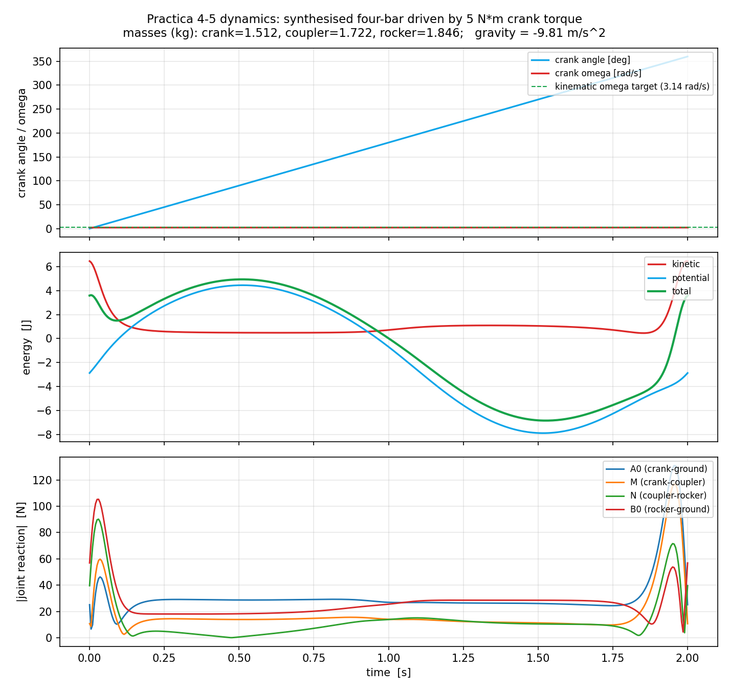
Years ago I had to make a practice