Programatic Mechanisms

Tl;DR

Same inputs, same outputs.

What’s stopping you to do programmatic mechanism analysis?

Intro

A multibody dynamics simulation framework written in MATLAB.

It solves the equations of motion for constrained mechanical systems — assemblies of rigid bodies connected by joints, acted upon by forces, and potentially in contact with surfaces.

#git clone https://github.com/JAlcocerT/mbsd
cd mbsd/2D-Kinematics
#python examples/slider_crank.py

#cd examples
# echo -e "file 'p1.mp4'\nfile 'p2.mp4'" > list.txt
# # 2. Join them
# ffmpeg -f concat -safe 0 -i list.txt -c copy output.mp4
# mpv "output.mp4"
python examples/pantograph.py

If you have been following my latest post about blender and bringin to life mechanism…

You could imagine that it was a matter of time for me to join these 2 worlds.

But first, as I have wood PCs, I needed to install tmux on my x300 to leave it thinking during the night via termix:

sudo apt update && sudo apt install tmux -y
#nano ~/.tmux.conf
loginctl enable-linger $USER
#tmux new -s cad_mbsd_render

git clone https://github.com/JAlcocerT/3Design
cd ./3Design/z-cadquery
make check #make help
#make scene-ui #this starts blender UI
#make all
tmux new-session -d -s cad "make all" #if you will be leaving this for the night
#tmux attach-session -t cad #to see hows going

After having the x300 processing at 100% and consuming 80-90W…

Then just some rsync magic will bring the generated files home:

rsync -avP jalcocert@192.168.1.2:/home/jalcocert/3Design/z-cadquery/render/slider_crank.mp4 .
#Then play it:
mpv slider_crank.mp4

So…

How hard is to make this work for any of the 2D kinematics I got ready?

2D Kinematics x Blender

As mentioned before, its about bridging the 2 worlds.

Why would this be impossible, if we are just stating:

1. A solid is infinitely rigid and 2 points always keep their distance constant
2. F=ma actually not yet. But later

The blender_scene.py is the one doing the cool rendered end result

One line to rule them all: change PRESET = “preview” to PRESET = “final” and the whole render pipeline switches (resolution, samples, motion blur, quality)

• FPS and FRAME_COUNT are now top-level variables alongside the file paths
• The render settings section now just reads from _p[…] — no more buried comments saying “change this for final render”
• Added a print line so you can confirm what preset is active when the script runs

Three presets now:

┌────────────┬────────────┬─────────┬─────────────┬───────────────────┐ │ Preset │ Resolution │ Samples │ Motion blur │ Use case │ ├────────────┼────────────┼─────────┼─────────────┼───────────────────┤ │ preview │ 1280×720 │ 8 │ off │ Quick local test │ ├────────────┼────────────┼─────────┼─────────────┼───────────────────┤ │ production │ 1920×1080 │ 16 │ off │ Overnight on x300 │ ├────────────┼────────────┼─────────┼─────────────┼───────────────────┤ │ final │ 3840×2160 │ 64 │ on │ Cinematic 4K

After some tinkering with blender, this was quite easy to do wit the fwk im building:

#git clone https://github.com/JAlcocerT/3D-Design
cd ./3D-Design/mbsd-to-render
#claude

i love this workflow and it works great for one example that we have for the slider crank. Could you now look at the folder mbsd-to-render where I have brought a 2d
  kinematics simulator for any mechanism and write a wiki-integration-cadquery.md with your understanding on how it works and what would be required to make there
  equivalents scripts that will interact with cadquery and blender programatically?

. How mbsd works — coordinate system, constraint types, solving pipeline, all 6 example mechanisms 2. The existing slider-crank pipeline — what data.json contract looks like today 3. What needs to be built per mechanism — 3 scripts each: - export_.py — runs the mbsd solver, converts 2D coords to 3D and writes data.json - cad_parts_.py — CadQuery parametric parts → STLs - blender_scene_.py — Blender scene builder (mostly copy of existing one) 4. Per-mechanism notes — four-bar, Geneva drive, Scotch yoke, pantograph specifics 5. Suggested folder layout and a shared/blender_utils.py idea to avoid duplication 6. The data contract — the data.json schema everything must agree on 7. Gap analysis table — what exists vs what needs building

The key insight is that the mbsd solver is already generic — you just need the 3 glue scripts per mechanism, using slider-crank as the template.

Will it work for any mechanism? Yes, with one caveat per mechanism type:

┌─────────────────────────┬───────────────────────────────────────────────────┐ │ Aspect │ Status │ ├─────────────────────────┼───────────────────────────────────────────────────┤ │ Kinematics solving │ ✅ fully generic, no changes needed │ ├─────────────────────────┼───────────────────────────────────────────────────┤ │ Velocity + acceleration │ ✅ same │ ├─────────────────────────┼───────────────────────────────────────────────────┤ │ data.json export │ ✅ same loop, just different body names │ ├─────────────────────────┼───────────────────────────────────────────────────┤ │ CadQuery parts │ ⚠️ manual per mechanism — each body needs a shape │ ├─────────────────────────┼───────────────────────────────────────────────────┤ │ Blender scene │ ⚠️ mostly copy-paste, just tune camera/lighting │ ├─────────────────────────┼───────────────────────────────────────────────────┤ │ 2D → 3D mapping │ ⚠️ same formula for all planar mechanisms │ └─────────────────────────┴───────────────────────────────────────────────────┘

So the only creative work per mechanism is:

1. Defining the geometry (link lengths, cross sections) for CadQuery
2. Tuning the camera in Blender to frame it well

cd ./3D-Design/mbsd-to-render/four-bar
#make help
make scene-ui #just to open blender UI and see whats coming on the laptop

And this also worked at the x300, generating:

cd ./3D-Design
#git pull
cd ./mbsd-to-render/four-bar
make all
rsync -avP jalcocert@192.168.1.2:/home/jalcocert/3Design/mbsd-to-render/four-bar/render/four_bar.mp4 .
mpv four_bar.mp4

2D Dynamics for MBSD

Its time for some: F=ma

cd ./mbsd/2D-Dynamics
#make help
make run-four-bar #make run-all
#cd /home/jalcocert/Desktop/mbsd/2D-Dynamics && timeout 120 bash -c 'cd examples && ../venv/bin/python dynamic_slider_crank.py 2>&1' | head -80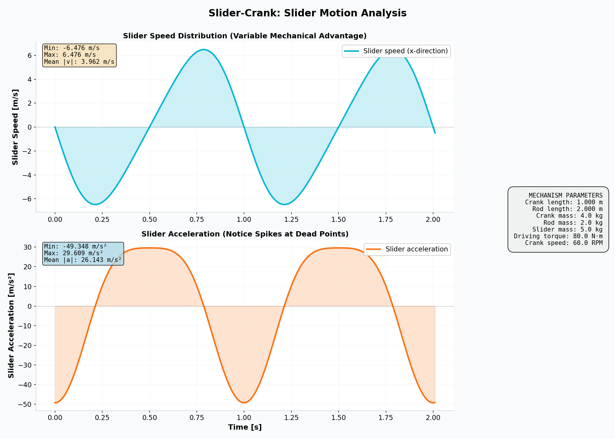

Just at 60rpm or 1 rev per second, the slider goes as fast as ~23km/h for some instants of time.

This one uses Lagrange, particularly: Constrained Lagrangian Mechanics

The Equation We Solve: M(q) @ a + ∇V(q) = Q_ext + C_q^T @ λ

Where:

• M(q) = Mass matrix (constant in reference coordinates)
• a = Acceleration vector (what we compute)
• ∇V(q) = Potential energy gradient (gravity effects)
• Q_ext = External forces (torques, springs, user input)
• C_q^T @ λ = Constraint reaction forces (the hidden part!)
• λ = Lagrange multipliers (automatic, varies with config)

Having said that, how about we forget about gravity for a sec?

#uv init --no-readme .

# Add packages from requirements.txt one-shot
uv pip install -r requirements.txt
#uv sync
make run-slider-crank-no-gravity

Conclusions

No 3D speeds and 3D forces for the mbsd model so far.

But dont worry, they are coming.

That one even has some fluid mechanics going on…

What would be the problem? :)

Upcoming questions to be resolved:

1. Whats the best angle for each V shape engine based on the vibrations?

V8 tend to be at 90 degrees, why?

2. The dynamics of the hip thrust exercise….

FAQ

The Lagrangian is Awesome

The Lagrangian is one of the most elegant concepts in physics. Here’s why it’s genius for obtaining equations of motion:

What is the Lagrangian?

The Lagrangian L is defined as:

$$L = T - V$$

where T is kinetic energy and V is potential energy.

Why It’s Genius

1. Unified Framework

Instead of tracking forces directly (which requires vector decomposition and can get messy with constraints), the Lagrangian uses energy—a scalar quantity. Scalars are simpler to work with than vectors.

2. Automatic Handling of Constraints

This is the real power. When you have constraints (like a pendulum fixed at one point, or a bead sliding on a wire), the Lagrangian naturally incorporates them through your choice of generalized coordinates.

You don’t need to calculate constraint forces explicitly—they disappear from the equations.

3. Elegant Mathematical Structure

The equations of motion come from the Euler-Lagrange equation:

$$\frac{d}{dt}\left(\frac{\partial L}{\partial \dot{q}}\right) - \frac{\partial L}{\partial q} = 0$$

This works for any coordinate system. Cartesian, polar, spherical, or some weird generalized coordinate—same equation.

4. Works in Any Reference Frame

Since energy is frame-independent (more precisely, frame-invariant for the dynamics we care about), you get equations of motion that are valid regardless of your choice of coordinates.

Simple Example: Pendulum

• Force approach: Calculate tension T, gravity components, resolve perpendicular to the rod → complicated
• Lagrangian approach: Use angle θ as your coordinate, write $L = \frac{1}{2}m\ell^2\dot{\theta}^2 - mg\ell(1-\cos\theta)$, apply Euler-Lagrange → done, you get the equation immediately

Why for Constrained Systems?

When you have constraints, the Lagrangian automatically “knows” which degrees of freedom matter.

You only have as many equations as you have actual degrees of freedom—constraint forces never appear in the equations.

This is exactly what makes it perfect for multibody dynamics like MBSD.

Systematic Choices for Computer Implementation

The Lagrangian is genius, but it can’t be fully automated—a human must choose the generalized coordinates and define the system.

A computer can’t magically know what degrees of freedom matter.

Generalized Coordinates: The Key Choice

For every rigid body in your system, you need to choose coordinates that describe its configuration. Some examples:

• Slider-crank mechanism: Use crank angle θ, slider position x, or maybe just θ if you enforce the kinematic constraint
• Pendulum: Use angle θ (1 DOF instead of 2 for x, y)
• Free-falling box: Use center of mass position (x, y) and orientation angle φ

What About Kinetic and Potential Energy?

Once you’ve chosen your coordinates, the rule is actually systematic:

• Kinetic Energy T: Always comes from the center of mass velocity of each body, plus rotational motion $$T = \sum_i \left(\frac{1}{2}m_i v_{cm,i}^2 + \frac{1}{2}I_i \omega_i^2\right)$$

• Potential Energy V: Comes from the center of mass height in gravity field, plus any other potential fields $$V = \sum_i m_i g h_{cm,i} + V_{springs}$$

So yes, always center of gravity (center of mass).

This is not a choice—it’s the only systematic way that works for rigid bodies.

What the Computer Does

Once you’ve defined:

1. Which generalized coordinates to use
2. The mass and inertia of each body
3. The constraints (if any)

Then the computer can:

1. Express T and V in terms of your coordinates
2. Compute the Lagrangian L = T - V symbolically
3. Apply Euler-Lagrange to get the differential equations automatically

This is exactly what tools like SymPy do in MBSD—you describe the system structure, and the computer derives the equations.

Why Reference Coordinates?

Simple: because they are sistematic.

I dont want to leave the program subject to human errors of mechanism understanding

At the cost of having to resolve more coordinates and equations.

Equations of Motion: What They Are and How to Solve Them

What Makes an Equation an “Equation of Motion”?

An equation of motion is any differential equation that describes how a system evolves in time.

More specifically:

1st order: $\frac{dx}{dt} = f(x, t)$ (velocity defined by position)

2nd order: $\frac{d^2x}{dt^2} = f(x, \dot{x}, t)$ (acceleration defined by position and velocity)

For mechanical systems, Newton’s 2nd law gives us 2nd-order differential equations: $$m\ddot{x} = F(x, \dot{x}, t)$$

The Lagrangian approach gives us these same equations, but derived automatically from energy rather than force: $$\frac{d}{dt}\left(\frac{\partial L}{\partial \dot{q}}\right) - \frac{\partial L}{\partial q} = 0$$

This is still a 2nd-order differential equation in disguise.

Why 2nd Order?

Physics requires two initial conditions: position and velocity.

Once you know where something is and how fast it’s moving, the future is determined.

Hence: 2nd-order equations.

Methods to Solve Equations of Motion

1. Analytical (Symbolic)

• Use: Simple systems (pendulum, spring-mass)
• Method: Solve the differential equations by hand or with SymPy
• Pro: Exact closed-form solutions
• Con: Only works for special cases (linear, simple geometries)
• Example: $\ddot{\theta} + \frac{g}{\ell}\sin\theta = 0$ → solution involves elliptic integrals

2. Numerical Integration

• Use: Complex systems, nonlinear dynamics, constraints
• Methods:
  • Runge-Kutta (RK4): Good balance of accuracy and speed
  • Symplectic integrators: Preserve energy over long simulations (important for mechanics!)
  • Implicit methods: For stiff systems where explicit methods become unstable
• Pro: Works for any system
• Con: Accumulates numerical error, requires small timesteps
• Example: MBSD uses numerical integration to simulate your mechanisms frame-by-frame

3. Linearization (for Small Motions)

• Use: When oscillations are small (θ ≈ 0)
• Method: $\sin\theta \approx \theta$, solve the simplified linear system
• Pro: Analytical solutions possible
• Con: Only valid near equilibrium

4. Energy Conservation (Special Cases)

• Use: Systems without friction or external damping
• Method: Use $E = T + V = \text{constant}$ to reduce problem dimension
• Pro: Reduces 2nd-order to 1st-order
• Con: Only works when energy is actually conserved

Why MBSD Uses Numerical Integration

For multibody systems with constraints, multiple degrees of freedom, and complex geometries, analytical solutions are impossible. Numerical integration is the only practical approach:

1. Lagrangian formulation gives you the differential equations
2. Numerical integrator steps through time: $q(t+\Delta t) = q(t) + \Delta t \cdot \dot{q}(t) + \ldots$
3. At each timestep, you evaluate accelerations from the equations of motion
4. Blender renders each timestep as a frame

This pipeline is why MBSD + Blender can animate any 2D mechanism you throw at it.