AI|BI Tools and PoCs with PyGWalker
Tl;DR
As a BIA, you might have to skip waiting for data engineering team to put together some pipeline.
You can build your visualizations into Grafana/GCP Looker/PowerBI/ whatever.
But if you know what to do with python…
+++ Created a quick data PoC with streamlit and PyGWalker.

Intro
It not just about old school BI Tools, or the well known propietary ones like Looker or PBi
Today, we will have a look to:
- ChartDB: A database diagrams editor that lets you visualize and design your database with a single query.
- Quix (wix-incubator): A powerful, open-source platform for data exploration and analysis.
- Querybook: Pinterest’s open-source big data ad-hoc query and visualization tool.
- Quix Streams: A Python library designed for building real-time data streaming applications.
And Also, to one custom AI/BI work that Ive been doing: Generating charts as a code via OpenAI Calls and render them directly into Streamlit.
Together with…PyGWalker
BI Tools
ChartBrew
Open-source web platform used to create live reporting dashboards from APIs, MongoDB, Firestore, MySQL, PostgreSQL, and more 📈📊
Which resonates with my recent post on BI Tools
ChartDB
I thought everything was done with LangChain querying DBs with LLMs in DAG mode.
Then I found this: https://github.com/chartdb/chartdb
agpl 3 | Database diagrams editor that allows you to visualize and design your DB with a single query.

DB2Rest
DB2Rest is blazing fast.
It has NO Object Relational Mapping (ORM) overhead, uses Single round-trip to databases, no code generation or compilation, and supports Database Query Caching and Batching.
#docker pull kdhrubo/db2rest:v1.6.4 #or docker pull kdhrubo/db2rest:latestApache v2 | Instant no code DATA API platform.
Connect any database, run anywhere. Power your GENAI application function/tools calls in seconds.
Conclusions
These are pretty interesting tools to consider in the analytics space.
As you can see, ChartDB has exploded recently in terms of popularity:
But how about the promised AI/BI part?
Lets have a look to a cool combo.
PyGWalker
What am I talking about: Streamlit x pygwalker
Give the users a webapp that they can play with tables / graph that does not require huge development!
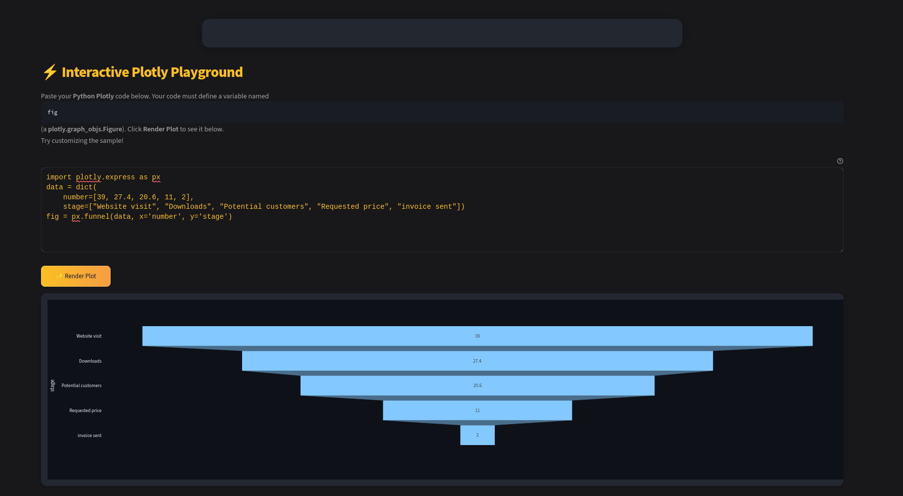
If you want to use actively AI to develop the dashboarding, consider LLM x Streamlit:
As can also render mermaidJS and plotly graphs with your aissistant, via streamlit webapp
You can also bring:
- QR Code Generation
- Plotly render inside Streamlit
- You can even modify DNS via this script
Remember about maps:
To run it, I will be using uv as a venv:
uv --version
#uv init #then pyproject.toml is created

#uv add streamlit plotly openai dotenv qrcode Pillow #creates the .venv
#uv add pygwalker==0.4.9 folium streamlit_folium
#uv add openpyxl

uv sync #creates/updates the uv.lock for repricability

uv run streamlit run main.py
#uv run streamlit run main.py  --env=./
Thats pretty much it (way faster than via pip install!)

Its also great to export your configured PyGWalker dashboard design into a compact JSON:
vis_spec = r"""{"config":[{"config":{"defaultAggregated":true,"geoms":["poi"],"coordSystem":"geographic","limit":-1,"timezoneDisplayOffset":0},"encodings":{"dimensions":[{"fid":"OLT","name":"OLT","basename":"OLT","semanticType":"nominal","analyticType":"dimension","offset":0},{"fid":"Latitude","name":"Latitude","basename":"Latitude","semanticType":"quantitative","analyticType":"dimension","offset":0},{"fid":"Longitude","name":"Longitude","basename":"Longitude","semanticType":"quantitative","analyticType":"dimension","offset":0},{"fid":"Geohash","name":"Geohash","basename":"Geohash","semanticType":"nominal","analyticType":"dimension","offset":0},{"fid":"SyntheticMapped","name":"SyntheticMapped","basename":"SyntheticMapped","semanticType":"nominal","analyticType":"dimension","offset":0},{"fid":"gw_mea_key_fid","name":"Measure names","analyticType":"dimension","semanticType":"nominal"}],"measures":[{"fid":"SyntheticLocationsforOLT","name":"SyntheticLocationsforOLT","basename":"SyntheticLocationsforOLT","analyticType":"measure","semanticType":"quantitative","aggName":"sum","offset":0},{"fid":"Viewers","name":"Viewers","basename":"Viewers","analyticType":"measure","semanticType":"quantitative","aggName":"sum","offset":0},{"fid":"Viewers_1","name":"Viewers_1","basename":"Viewers_1","analyticType":"measure","semanticType":"quantitative","aggName":"sum","offset":0},{"fid":"Viewers_14","name":"Viewers_14","basename":"Viewers_14","analyticType":"measure","semanticType":"quantitative","aggName":"sum","offset":0},{"fid":"KPI_1","name":"KPI_1","basename":"KPI_1","analyticType":"measure","semanticType":"quantitative","aggName":"sum","offset":0},{"fid":"KPI_14","name":"KPI_14","basename":"KPI_14","analyticType":"measure","semanticType":"quantitative","aggName":"sum","offset":0},{"analyticType":"measure","fid":"gw_SkCP","name":"KPI_Color","semanticType":"quantitative","computed":true,"aggName":"sum","expression":{"op":"expr","as":"gw_SkCP","params":[{"type":"sql","value":"case when KPI_14 > 0.07 then 1 else 0 end"}]}},{"fid":"gw_count_fid","name":"Row count","analyticType":"measure","semanticType":"quantitative","aggName":"sum","computed":true,"expression":{"op":"one","params":[],"as":"gw_count_fid"}},{"fid":"gw_mea_val_fid","name":"Measure values","analyticType":"measure","semanticType":"quantitative","aggName":"sum"}],"rows":[],"columns":[],"color":[{"analyticType":"measure","fid":"gw_SkCP","name":"KPI_Color","semanticType":"quantitative","computed":true,"aggName":"sum","expression":{"op":"expr","as":"gw_SkCP","params":[{"type":"sql","value":"case when KPI_14 > 0.07 then 1 else 0 end"}]}}],"opacity":[],"size":[],"shape":[],"radius":[],"theta":[],"longitude":[{"fid":"Longitude","name":"Longitude","basename":"Longitude","semanticType":"quantitative","analyticType":"dimension","offset":0}],"latitude":[{"fid":"Latitude","name":"Latitude","basename":"Latitude","semanticType":"quantitative","analyticType":"dimension","offset":0}],"geoId":[],"details":[{"fid":"KPI_1","name":"KPI_1","basename":"KPI_1","analyticType":"measure","semanticType":"quantitative","aggName":"sum","offset":0},{"fid":"KPI_14","name":"KPI_14","basename":"KPI_14","analyticType":"measure","semanticType":"quantitative","aggName":"sum","offset":0}],"filters":[],"text":[]},"layout":{"showActions":false,"showTableSummary":false,"stack":"stack","interactiveScale":false,"zeroScale":true,"size":{"mode":"auto","width":800,"height":600},"format":{},"geoKey":"name","resolve":{"x":false,"y":false,"color":false,"opacity":false,"shape":false,"size":false},"scaleIncludeUnmatchedChoropleth":false,"showAllGeoshapeInChoropleth":false,"colorPalette":"darkGreen","useSvg":false,"scale":{"opacity":{},"size":{}}},"visId":"gw_-1jR","name":"Chart 1"}],"chart_map":{},"workflow_list":[{"workflow":[{"type":"transform","transform":[{"key":"gw_SkCP","expression":{"op":"expr","as":"gw_SkCP","params":[{"type":"sql","value":"(CASE WHEN (\"KPI_14\" > (0.07)) THEN (1) ELSE (0) END )"}]}}]},{"type":"view","query":[{"op":"aggregate","groupBy":["Longitude","Latitude"],"measures":[{"field":"gw_SkCP","agg":"sum","asFieldKey":"gw_SkCP_sum"},{"field":"KPI_1","agg":"sum","asFieldKey":"KPI_1_sum"},{"field":"KPI_14","agg":"sum","asFieldKey":"KPI_14_sum"}]}]}]}],"version":"0.4.9"}"""Remember that you can also use Plotly/ChartJS/ApexCharts inside streamlit: