Electronics 101
Tl;DR
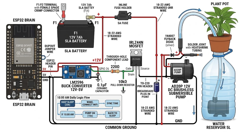
Prep-work for watering plants :)
Intro
You might have tinkered with IoT
But without really understanding the under lying layer.
This sits on top of Electromagnetism, yet below IoT and messaging protocols.
Circuit Boards Design
Everything is…code.
Same applies to circuit boards:
MIT | Design circuit boards with code! ✨ Get software-like design reuse 🚀, validation, version control and collaboration in hardware; starting with electronics ⚡️
Write hardware like software. atopile is a language, compiler, and toolchain for electronics—declarative .ato files, deep validation, and layout that works natively with KiCad.
A come back to electronics
After drafting several ideas around electronics, I made some samples with simulations and understanding.md to get the confidence back
Conclusions
So…mbsd is code, CAD and blender renders are code:
Electronics board design…yep, also code from now on.
#git init && git add . && git commit -m "Initial commit: Starting electronics 101" && gh repo create electronics-101 --private --source=. --remote=origin --push
#uv init
#uv add -r requirements.txt
#uv sync
#cd sample-pyscipe
uv run main.py

#make run #requires .env.local
You know whats coming
right?
Wait…if this is code…can it be animated with remotion?
In this folder i have added a pyscipe that simulates a particular circuit
  (see the makefile entries), I have also added a video remotion folder, with
  agents skills you can use. My idea is to generate a video animation of what
  happens in that given circuit with the intensities and voltages. Do you need
  to clarify sth?
Ive dare to generate such explanatory video: do you beliave you need that Diode now? :)
#git clone VideoEditingRemotion
cd ./remotion-electronics/my-video
# npx remotion render MosfetProtected mosfet_protected.mp4
#npx remotion render MosfetUnprotected mosfet_unprotected.mp4

npx remotion render SchematicKickback schematic_kickback.mp4#sudo apt update && sudo apt install ffmpeg
ls *.mp4 | sed "s/^/file '/; s/$/'/" > file_list.txt #add .mp4 of current folder to a list
ffmpeg -f concat -safe 0 -i file_list.txt -c copy output_video.mp4 #original audioToy models can NOT predict.
No model is perfect, reality is far to complex.
Its just that some are based on garbage and produce (surprise) more non sense garbage.
Why would someone pay you if you can just overfit past and give just a vague range of possibilities for the future?
Will the mosfet be fried, yes or no?
No more: will I get an unexpected quickback due to transitory behaviour?

Just…simulate: see thats going to happen, before it happens
git clone https://github.com/JAlcocerT/electronics-101
#cd ./electronics-101/sample-pyscipe
uv run main.py --only mosfet --scenario compare   # overlay: with vs without diode
The Meta-Lesson
All of these curiosities point to one theme:
Linear analysis predicts steady state. Nonlinearities dominate transients.
- The motor inrush looks linear for 100µs, then saturation takes over.
- The capacitor impedance is Ohmic for DC, but ESR-dominated for 150kHz ripple.
- The MOSFET is a resistor at steady state, but an avalanche diode in stress.
- The flyback diode’s nonlinearity is the only thing preventing the circuit from killing itself.
Real circuit design is about:
- Identifying which nonlinearities matter (flyback diode → essential; parasitic R → helpful)
- Ensuring they trigger safely (clamp at 12.7V, not 101.7V)
- Controlling their speed (ESR damping, gate slew rate)
- Testing edge cases (cold start, aged battery, old capacitors)
That’s why the simulations included these three scenarios: protected, unprotected, and compare.
The math alone doesn’t tell you the story.
You have to see it.
FAQ
About Electronical Simulations
Interesting engineering tools:
- KiCad
- Atopile
- PySpice: the discovery of today :)
To simulate the behaviour of ESP32, picoW, even arduino’s we have Velxio: https://github.com/davidmonterocrespo24/velxio
Quick IoT Samples
git clone https://github.com/JAlcocerT/RPi
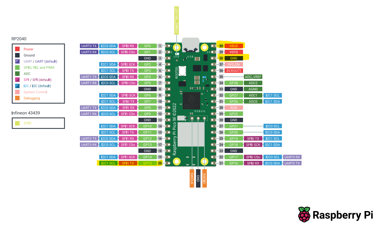
cd ./RPi/Z_MicroControllersWith the PicoW
cd ./RPiPicoW/DHT22For something more advance, see how the PicoW can read and send DHT22 data via MQTT
#cd ..
cd ./MQTT-DHT22
Remember about going to http://192.168.1.2:18083/#/clients and later to http://192.168.1.2:18083/#/websocket so you can subscribe, for example to pico/temperature/dht22 as explained with details here
#git clone
#cd ./Home-Lab/emqx
#docker compose up -d
# Check if the container is running
docker ps | grep emqx

# Watch EMQX logs live
docker logs emqx -f
Connect to the UI via:
http://192.168.1.11:18083
Or if you prefer a quick CLI way to check the pushed data:
mosquitto_sub -h 192.168.1.2 -t "pico/#" -vWith the ESP32: its very important to see which language was installed, as Thonny will just work with MicroPython!
*So go ahead and install arduinoIDE like so
#choco install arduinoide
#pnputil /enum-devices /class Ports
#git clone https://github.com/JAlcocerT/RPi
# cd ./RPi/Z_MicroControllers/ESP32/esp32-c
Select ESP32-WROOM-DAESP32 Dev Module + CTRL + U to compile the sketch esp32-internal-temp-mqtt.cpp into the board.
I got a ESP32 DevKitV1 printed on the back of it, despite on the chip it says ESP32 wroom 32
See your MQTT data flowing to the server:
mosquitto_sub -h 192.168.1.2 -t "esp32/#" -v 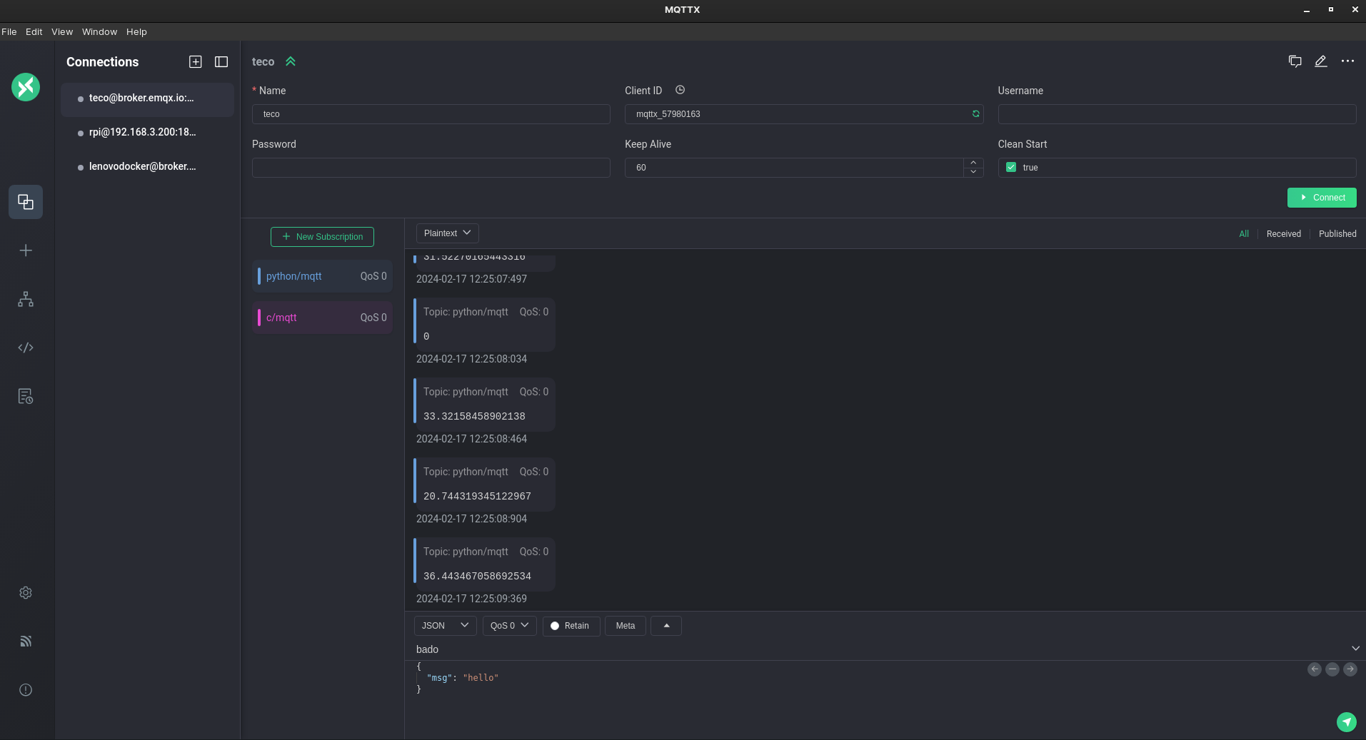 MQTT and Messaging Protocols
 Micro-Controller Scripts
To send DHT11 information via mqtt with the esp32, just: install Adafruit Unified Sensor & DHT sensor library for ESPx at arduino ide -> Tools -> Manage Libraries
mosquitto_sub -h 192.168.1.2 -t "esp32/#" -v
#mosquitto_sub -h 192.168.1.2 -t "esp32/temperature/dht11"
After compiling and uploading this one, the data is flowing CTRL+shift+mas expected :)
| Choice | GPIO Numbers | Why? |
|---|---|---|
| Best | 4, 14, 25, 26, 27, 32, 33 | No special boot functions; very stable. |
| Okay | 12, 13, 15 | Strapping pins; might cause boot/flash issues. |
| Bad | 34, 35, 36, 39 | Input only. Cannot trigger the DHT11. |
| Avoid | 0, 1, 2, 3 | Critical for booting and USB communication. |
Made one upgrade to the simple dht webapp, so that now it can plot both sensors:
# stop old sessions
#tmux kill-session -t mqtt
#tmux kill-session -t webapp
# verify they're gone
#tmux ls
#git clone https://github.com/JAlcocerT/RPi
#git pull
cd ./RPi/Z_MicroControllers/dht-webapp
#  tmux new-session -d -s mqtt 'cd ~/dht-webapp && uv run mqtt_to_db.py'
#   tmux new-session -d -s webapp 'cd ~/dht-webapp && uv run uvicorn main:app --host
#   0.0.0.0 --port 8077'
tmux new-session -d -s mqtt 'uv run mqtt_to_db.py'
#uv run uvicorn main:app --host 0.0.0.0 --port 8077
tmux new-session -d -s webapp 'uv run uvicorn main:app --host 0.0.0.0 --port 8077'
This will give you the trend and the last value read in real time:
docker exec -it timescaledb psql -U pico -d sensors -c \
  "SELECT DISTINCT ON (topic)
          topic,
          ROUND(value::numeric, 2) AS value,
          ts
   FROM readings
   WHERE topic IN (
     'pico/temperature/dht22',
     'pico/humidity/dht22',
     'esp32/temperature/dht11',
     'esp32/humidity/dht11'
   )
   ORDER BY topic, ts DESC;"
ESP32 vs PicoW Consumption
I could not avoid to make a quick experiment around power consumption.
How long would each of these micocontrollers be sending data via MQTT before consuming the same battery?
In theory, the a PicoW should be the winner.
The Pico W is roughly 2× more efficient than the ESP32 on the same battery — mainly because its WiFi chip (CYW43439) draws less than the ESP32’s radio at idle.
The DHT11/22 itself contributes almost nothing to consumption.
#docker exec -it timescaledb psql -U pico -d sensors -c "SELECT DISTINCT topic FROM readings LIMIT 10;"
docker exec -it timescaledb psql -U pico -d sensors -c \
    "SELECT time_bucket('1 hour', ts) AS hour, AVG(value) FROM readings WHERE topic =
  'pico/temperature/dht22' GROUP BY hour ORDER BY hour DESC LIMIT 24;"

docker exec -it timescaledb psql -U pico -d sensors -c \
  "SELECT time_bucket('1 hour', ts) AS hour,
          topic,
          ROUND(AVG(value)::numeric, 2) AS avg_value
   FROM readings
   WHERE topic IN (
     'pico/temperature/dht22',
     'pico/humidity/dht22',
     'esp32/temperature/dht11',
     'esp32/humidity/dht11'
   )
   AND ts > NOW() - INTERVAL '24 hours'
   GROUP BY hour, topic
   ORDER BY topic, hour DESC;"
Lets check this out.
- Connected the PicoW a Saturday 11pm to a 4000mAh battery
- When did the data stop flowing to TimescaleDB? Expected ~3/4 days, real: 21 hours
Maybe the battery was no 4000mAh at all?
for a relative comparison with the esp32, it doesnt matter
So i recharged the battery and tried with the ESP+dht11 setup
Surprisingly, the ESP32 just lasted ~11h instead of ~21h
For another time, ill be testing the deep sleep option to see how it improves
Also, I have to test using Zigbee instead of Wifi as it should also lower the power consumption
Interesting Tools
uv add schemdraw #https://github.com/cdelker/schemdraw/DC motors are simpler to control (just vary voltage) but brushed ones wear out and BLDC needs a 3-phase inverter AC motors (induction) are dumb-rugged — no electronics needed, just plug into the wall, but speed control requires a VFD Modern trend: AC is being eaten by BLDC everywhere efficiency or precision matters (EVs, drones, modern HVAC, e-bikes)
| Tool | Use | License |
|---|---|---|
| Ngspice | The SPICE engine you’re already using | BSD |
| PySpice | Your Python wrapper | GPL |
| KiCad | Schematic + PCB design — fully production-grade | GPL |
| Qucs / QucsStudio | GUI circuit simulator (Qucs is FOSS; QucsStudio is freeware) | GPL / freeware |
| GNU Octave | MATLAB-compatible numerical computing | GPL |
| Scilab + Xcos | Simulink-like block diagram simulation | GPL |
| OpenModelica | Multi-physics modelling (electrical, mechanical, thermal) | OSMC-PL |
| OpenDSS | Distribution-grid power flow & analysis (EPRI) | BSD |
| SAM (System Advisor Model) | NREL’s solar/wind/storage simulator — the open-source PVsyst alternative | BSD |
| pvlib-python | Solar modelling library — irradiance, panel models, MPPT | BSD |
| PySAM | Python bindings for SAM | BSD |
| Verilog-A in Ngspice | Behavioural device modelling | BSD |
LPF
A low-pass filter lets low frequencies through unchanged and attenuates (reduces) high frequencies.
INPUT signal:    a mix of low (e.g. 1 Hz) and high (e.g. 10 kHz) frequencies
LPF (f_c = 100 Hz)
OUTPUT signal:   the 1 Hz components are still there at full strength
                 the 10 kHz components are squashed to ~1% of their input
The filter has one parameter: the cutoff frequency f_c. Below f_c the filter is “open”; above f_c it progressively closes.
From the L4:
In the watering BRD (sample-pyscipe) the smoothing cap on the 5 V rail is a tiny LPF.
The 0.1 µF bypass cap forms an LPF with the trace inductance, blocking high-frequency noise from reaching the ESP32.
Every well-designed power rail has an LPF on it, often hidden in the layout.
| Where | What the LPF does | Typical f_c |
|---|---|---|
| Audio bass-only output | Sends only the low frequencies to a subwoofer | 80-150 Hz |
| ADC anti-aliasing | Blocks frequencies above f_sample / 2 to prevent aliasing | half the sample rate |
| Sensor smoothing | Removes high-frequency electrical noise from a slow signal (temperature, soil moisture) | 1-10 Hz |
| Power supply ripple removal | The output cap of a buck converter is part of an LPF — passes DC, blocks 150 kHz switching | well below f_switch |
| Servo / control loops | Smooths PID output to avoid jitter on the actuator | depends on system bandwidth |
| MOSFET gate slew control | Slows a switching edge from ns to µs to reduce EMI radiation | RC chosen for desired dV/dt |
| Audio EQ “treble cut” | Reduces shrillness | 5-10 kHz |
| Video composite signal | Limits chroma bandwidth to ~1 MHz to keep the carrier clean | 1.3 MHz (PAL) |
What is a high-pass filter (HPF)?
A high-pass filter is the LPF’s mirror: it lets high frequencies through unchanged and blocks low frequencies (including DC).
INPUT signal:    a mix of slow drift (DC, 0.1 Hz) and audio (1 kHz)
HPF (f_c = 100 Hz)
OUTPUT signal:   the slow drift is gone — the cap blocks DC
the 1 kHz audio is preserved| Where | What the HPF does | Typical f_c |
|---|---|---|
| AC coupling between op-amp stages | Strips out DC offsets so the next stage’s bias isn’t disturbed | 1-10 Hz |
| Sensor offset removal | A slow-varying baseline (electrode polarisation, thermal drift) gets stripped, leaving the fast signal of interest | 0.1-1 Hz |
| EKG amplifier | Removes 0.05 Hz baseline wander while passing the 1-40 Hz heartbeat content | 0.05 Hz |
| Edge detection / differentiator | At very high f_c relative to signal, the HPF behaves like d/dt | varies |
| DC-blocking on a coax line | The cap in series with an antenna feed prevents DC current paths | depends on RF band |
How do I pick f_c for my application?
Two rules of thumb:
For a SIGNAL filter (e.g. removing noise from a sensor reading): put f_c at least 10× higher than the highest frequency of interest. A 1 Hz sensor signal? Use f_c ≥ 10 Hz. Why “10×”? Because at f_c the signal is already attenuated by 3 dB (30%), which you usually don’t want. At f_c / 10 the attenuation is negligible.
For a NOISE filter (e.g. blocking switching noise): put f_c at least 10× lower than the noise frequency. A 150 kHz buck converter ripple? Use f_c ≤ 15 kHz. At f_c × 10 (one decade past) you’ve already attenuated by 20 dB (factor of 10) — usually plenty.
The hard cases are when signal and noise live in adjacent bands. That’s when you reach for higher-order filters (L4 plot 3 buffered cascade), or active filter topologies, or eventually digital filtering after an ADC.
What does “dB” really mean?
dB (decibel) is a logarithmic ratio:
gain in dB = 20 · log₁₀(V_out / V_in)
or
gain in dB = 10 · log₁₀(P_out / P_in)
The factor of 20 (vs 10 for power) is because P ∝ V², so log(V²) = 2·log(V).
They give the same dB number for the same physical situation.
Useful conversions to memorize:
| Ratio | dB |
|---|---|
| 1× | 0 dB |
| √2 ≈ 1.41 | +3 dB (doubled power) |
| 2× | +6 dB |
| 10× | +20 dB |
| 100× | +40 dB |
| 1000× | +60 dB |
The reason engineers use dB: a multi-decade frequency response would be impossible to read on a linear scale. dB compresses 6 orders of magnitude into 120 dB — manageable.
What’s the difference between a “first-order” and “second-order” filter?
The order is the number of independent energy-storing elements in the filter:
- 1st order: 1 capacitor (or 1 inductor). Slope = -20 dB/dec, max phase shift 90°.
- 2nd order: 2 caps, or 1 cap + 1 inductor. Slope = -40 dB/dec, max phase shift 180°. Can have a resonance peak (Q > 0.5).
- n-th order: n energy-storing elements. Slope = -20·n dB/dec. n × 90° max phase shift.
Higher order = sharper transition between passband and stopband, at the cost of more parts and more chance for things to go wrong (oscillation, peaking, group delay distortion).
The buffered cascade in plot 3 is a 2nd-order LPF.
It’s two 1st-order stages, isolated by a buffer, so their transfer functions multiply.
Where does the 2π come from in f_c = 1/(2πRC)?
Conversion between angular frequency ω (in rad/s) and ordinary frequency f (in Hz):
ω = 2π · fA sine wave at 1 Hz completes 2π radians of phase per second. The “natural” frequency for the math is ω, but humans measure in Hz, so we live with the 2π. It’s a unit conversion, nothing more.
If you ever see ω_c = 1/(RC) (no 2π), it means we’re working in radians per second instead of cycles per second. Same circuit, same f_c, just expressed in rad/s.
What about LC filters? When do you use those instead of RC?
When you need a sharp cutoff (high Q) or low loss in the passband.
RC filters can only achieve Q = 0.5 and always dissipate signal energy in R.
LC filters can have Q > 100 with no resistors at all (just unavoidable parasitics).
Trade-offs:
| RC | LC |
|---|---|
| Cheap, small, no inductors | Inductors are bulky, expensive, and pick up EMI |
| Q ≤ 0.5 | Q > 0.5 possible (resonance, ringing) |
| Always damped | Can ring or oscillate without R for damping |
| OK at any frequency | Below ~10 kHz, inductors get huge; above ~1 GHz, parasitics dominate |
In the watering BRD, the buck converter’s L+C output is an LC filter.
The Q is moderate (resistance from MOSFET Rds(on), inductor DCR, ESR of cap) and the cutoff is well below the 150 kHz switching frequency, giving clean Vout.