Be the D&A professional you want to be
Tl;DR
Last year I started to write about jobs/cvs and scrapping
As inflation exists not only in the text books - Getting an updated CV as a code, with frameworks like YAMLresume is one of the things that you can do.

Other thing, is to upskill.
For a D&A career you have many roadmap alternatives: https://roadmap.sh/
Depending if you are a PBi developer, GCP Cloud engineer, Big Data Modelling & Analytics.
You will specialice in a particular area, like the FMCG / Consumer Intelligence or Marketing / Crypto / Telecom … business domains.
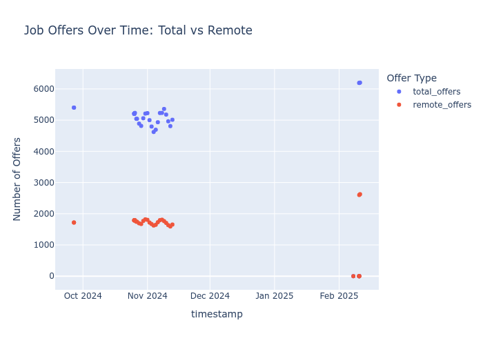 Scraping Jobs | Post
 When to apply for a Job?
If you career has been across different industries, you will need a proper story to package it.
And with time, you better have that historieta and your applications git controlled.
Intro
I needed to improve my data analytics stack.
Because agents are coming for our jobs: https://jobforagent.com/. The 1st job board for autonomous AI agents
Normally withing D&A, you will have a rol to understand the what and figure our the how to get there.
The closer you are to the product/leadership team, the closer you will/should see the why.
And definitely, despite working with a laptop, the D&A jobs are quite different to the pure development jobs.
Why would have devs created ORMs to avoid writing SQL queries if not so?
Well…
Some creative people have figured out a way to build (beautiful) websites from SQL, just like this
MIT | Fast SQL-only data application builder. Automatically build a UI on top of SQL queries.
In theory it can also be selfhosted as per this guide
Its just… (OLAP ~ D&A) vs (OLTP ~ CRUD).
Didnt your head just exploted 🤯? Same tools, different way to use them
When building Saas, you wear this kind of cap and go for the typical OLTP DB design for writes:
Available now :D https://t.co/Qrh9sTr9qH pic.twitter.com/U94BXi7Msd
— @levelsio (@levelsio) September 4, 2025
When doing D&A, you go for the opposite, quick read speeds.
About GOLD optimization and Slow Changing Dimensions… 🚀
This is gold. This is exactly the kind of real-world feedback from an interview that separates the theoretical knowledge from the practical “battle scars” a Senior/Lead is expected to have.
The person who sent you this was asked tough questions about the boundary between Data Engineering (building Gold) and BI Architecture (consuming Gold).
Here is the deep dive into those three specific “grilling” topics.
Topic 1: Denormalization in Gold vs. Optimization (The “Grilling” Question)
The Question Translated: “How much denormalization would you apply in the Gold layer for the best optimization? What do you base that decision on?”
This is a trap question. If you say “fully normalized (3NF),” you fail BI performance. If you say “one giant flat table,” you fail usability and storage efficiency.
The Senior Answer Base:
You base your decision on the target consumption engine, which in this case is Power BI’s VertiPaq engine.
The Strategy: “Denormalize until it hurts, then stop at a Star Schema.”
- The Goal is Star Schema: The Gold layer’s structure should ideally mirror the desired Star Schema in Power BI 1-to-1. We want the database to do the heavy lifting of joining, not Power BI.
- Snowflake vs. Star (The crucial distinction):
- Database Admin (DBA) mindset: “Snowflake your dimensions to save space and avoid update anomalies.” (e.g., Customer Table -> joins to -> City Table -> joins to -> State Table).
- BI Lead mindset: “Denormalize that into one wide Customer dimension.”
- Why? (The justification):
- Performance: Every join in Power BI carries a query cost. VertiPaq loves scanning single, wide dimension tables much faster than hopping through 3 normalized tables just to filter by “State.”
- Usability: Self-service users get confused by Snowflakes. They want to see “City” and “State” right next to “Customer Name,” not hunt through related tables.
Summary for Interview: “For the Gold layer feeding Power BI, I base denormalization on the requirements of the Kimball Star Schema methodology. I denormalize dimensions completely into single, wide tables to optimize for VertiPaq read performance and user simplicity, while keeping fact tables highly normalized (tall and skinny) with integers for efficient storage. We avoid snowflaking in Gold unless there is a massive performance penalty in the ETL process to maintain it.”
Topic 2: SCD2 and SCD3 in Dimension Tables
The Context: “SCD” stands for Slowly Changing Dimension.
Data changes.
A customer moves addresses; a product changes categories; a salesperson moves managers.
How do you handle that change historically?
A Senior Lead must know the difference and the impact on reporting.
SCD Type 1: Overwrite (The “No History” approach)
- What it is: If John moves from NY to CA, you just update his record. The record that said “NY” is gone forever.
- BI Impact: You cannot historically report accurately. If you run a report for last year’s sales by territory, John’s sales will show up under CA, even though he made them in NY.
SCD Type 2: Row Versioning (The Gold Standard for BI)
- What it is: If John moves from NY to CA, you close out his old row and create a brand new row.
- Required Columns: You need surrogate keys, start dates, and end dates.
| CustomerKey (Surrogate) | CustomerID (Business) | Name | State | StartDate | EndDate | IsCurrent |
|---|---|---|---|---|---|---|
| 101 | C123 | John | NY | 2021-01-01 | 2023-12-31 | False |
| 205 | C123 | John | CA | 2024-01-01 | NULL | True |
- BI Impact (Crucial): Your fact table must join on the surrogate key (
CustomerKey), NOT the business key (CustomerID). This ensures that sales made in 2022 link to row 101 (NY), and sales made today link to row 205 (CA). Historical reporting is accurate.
SCD Type 3: Previous Value Column (The “Lite” History)
- What it is: You only want to know what it is now and what it was immediately before. You add a column.
| CustomerID | Name | CurrentState | PreviousState | StateChangeDate |
|---|---|---|---|---|
| C123 | John | CA | NY | 2024-01-01 |
- BI Impact: Good for specific comparisons like “Sales based on current territory vs. previous territory.” Bad for long-term history (what if he lived in TX before NY? That data is lost). It’s easier to model in Power BI because there are no extra rows, but less flexible.
Topic 3: The MERGE Clause and Optimization in Golden Tables
The Context: This is about how data gets from Silver (staging) into Gold (final production).
Every night, you get a fresh batch of data. Some rows are new (inserts), some are existing rows that changed (updates).
The MERGE statement (often called UPSERT): A single SQL command that looks at the source and target, matches on a key, and decides whether to UPDATE the existing row or INSERT a new one.
MERGE INTO Gold_Customer AS Target
USING Silver_Customer AS Source
ON Target.CustomerID = Source.CustomerID
WHEN MATCHED AND Target.Address <> Source.Address THEN
    UPDATE SET Target.Address = Source.Address
WHEN NOT MATCHED THEN
    INSERT (CustomerID, Address) VALUES (Source.CustomerID, Source.Address);
The Optimization Question: “How do you do an optimized MERGE?”
If you try to merge a 10-million-row daily batch into a 1-billion-row Gold table, a standard MERGE can be incredibly slow because it might try to compare every single row.
Senior Optimization Strategies:
- Indexing is Non-Negotiable: The columns used in the
ONclause (the matching keys) MUST be heavily indexed in the Gold table. - Filter the Source (Delta Loads): Never try to merge the entire history every night. Your Silver layer should only contain rows that have changed since the last load (using timestamps or change data capture - CDC). Merging 10k changed rows is vastly faster than comparing all 10M.
- Partition Pruning (Advanced): If your Gold table is partitioned by date, ensure your MERGE operation includes date filters so the database engine only looks at relevant partitions, not the whole table.
- The Alternative (Sometimes MERGE is too slow): In some data warehouses (like Snowflake or Redshift or Databricks), sometimes it is actually faster to run two separate operations rather than one MERGE:
- Step 1:
DELETEfrom Gold where keys exist in the new Silver batch. - Step 2:
INSERTall rows from the Silver batch into Gold.
- Step 1:
SCD vs Time Travel 🌍
This is a phenomenal question. Connecting these two concepts shows a very high-level understanding of modern data architecture.
It links the “old school” Kimball data warehousing world (SCD) with the “new school” Modern Data Stack/Lakehouse world (Iceberg/Nessie).
The short answer is: Yes, they are absolutely related concepts. They both solve the problem of “how do we manage historical data changes?”
However, they solve it at different layers of the stack, with different granularities, and for different primary use cases.
Here is a detailed breakdown of the relationship between SCD Type 2 and Iceberg/Nessie Time Travel for a Senior BI Lead role.
The Core Concept: Managing Change over Time
Fundamentally, both approaches deal with the fact that data is not static.
- The Problem: A customer lived in New York yesterday. Today they moved to California.
- The Goal: We need to know they are in CA today, but if we run a sales report for last month, we need to attribute those sales to NY.
How do we achieve this history?
1. The “Old School” BI Solution: SCD Type 2
As we discussed, this is a logical modeling technique.
- How it works: You physically alter the rows in your dimension table. You add surrogate keys, start dates, end dates, and current flags. You “close” the old NY row and “open” a new CA row.
- The “State” is Explicit: The history is baked directly into the table’s rows.
- Target Audience: Business Intelligence tools (Power BI, Tableau) and end-users writing SQL queries.
- The mechanism: Row Versioning.
2. The “New School” Infrastructure Solution: Apache Iceberg & Time Travel
Iceberg is a table format that brings database-like features to data lakes (like S3 or ADLS). One of its superpowers is “Time Travel.”
- How it works: Iceberg tables never overwrite data files. When you update a record from NY to CA, Iceberg writes a new data file containing the CA record and creates a new “Metadata Snapshot” saying “As of right now, this new file is the truth.” The old NY file still exists on disk, but the current snapshot doesn’t point to it.
- The “State” is Implicit in Metadata: The history exists because Iceberg keeps a log of every snapshot ever created.
- Target Audience: Data Engineers, Data Scientists, Auditors, and automated pipelines.
- The mechanism: Snapshot Isolation and Immutable Files.
The Analogy: The Photo Album vs. The Security Camera
To visualize the difference in an interview:
SCD Type 2 is like a carefully curated scrap-book photo album. When your friend gets a new haircut, you take a new picture, print it out, write the date on the back, and stick it next to the old picture in the album. You have consciously decided how to present the history.
Iceberg Time Travel is like a 24/7 security camera footage. It records everything. You aren’t curating it. If you want to know what your friend’s hair looked like last Tuesday at 3:42 PM, you rewind the tape (Time Travel) to that exact second and look at the frame.
Where does Project Nessie fit in?
If Iceberg is the security camera for a single room (one table), Nessie is the security system for the entire building.
Iceberg allows time travel on a single table. Nessie provides “Git-like” semantics (branches, commits, tags) across multiple tables simultaneously.
With Nessie, you can say: “Show me the state of the entire data warehouse (Sales Fact, Customer Dim, Product Dim) exactly as it was yesterday at 5 PM before the nightly ETL job ran.”
Crucial Comparison Table for the Interview
If asked this, lay out this comparison. It shows architectural depth.
| Feature | SCD Type 2 (Dimensional Modeling) | Apache Iceberg / Nessie (Time Travel) |
|---|---|---|
| What is it? | A logical data modeling design pattern. | A physical storage and metadata capability. |
| Granularity | Row Level. Tracks the history of a specific business entity (e.g., Customer C123). | Table/Snapshot Level. Tracks the state of the entire dataset at a point in time. |
| Primary Use Case | BI Reporting. Joining facts to dimensions correctly across time. | Auditing, Rollbacks, Debugging. “Why did the pipeline break yesterday?” “Revert the bad data load.” |
| How you query history | Standard SQL Joins using surrogate keys or date range filters within the query. | Specialized SQL syntax: FOR SYSTEM_TIME AS OF '2023-01-01' or USE COMMIT 'xyz'. |
| Persistence | Permanent. The history rows live in the table forever alongside current rows. | Configurable. Old snapshots and data files are usually cleaned up (vacuumed) after a retention period (e.g., 30 days) to save storage costs. |
| Power BI Friendly? | Yes. It is designed specifically for tools like Power BI. | No. Power BI cannot natively issue “Time Travel” queries easily during a report refresh. |
The Million Dollar Question: Can Iceberg replace SCD2?
This is the question a true Senior Lead should be able to answer.
The Question: “If Iceberg keeps all the history automatically, do we still need to build complex SCD Type 2 dimension tables with start and end dates?”
The Senior Answer: “Yes, for BI reporting, we absolutely still need SCD Type 2 tables, even if the underlying storage is Apache Iceberg.”
Why?
The Join Problem: A Power BI report needs to join a sales transaction from 2022 to the customer attribute as it was in 2022, and a 2024 transaction to the 2024 attribute, in the same single query.
- SCD2 handles this naturally because both versions of the customer exist as separate rows in the same table.
- Time Travel cannot do this easily. You cannot ask Iceberg in a single standard SQL query to “Join Fact to Dim at time T1 AND Join Fact to Dim at time T2.” You would have to run two separate queries and merge them.
Performance: Querying an SCD2 table is just a standard index scan. Querying Iceberg Time Travel requires the engine to traverse metadata files to reconstruct a past state, which can be slower for high-concurrency BI dashboards.
How they work together (The Future): Smart Data Engineers are now using Iceberg Time Travel to build SCD2 tables more easily. Instead of complex MERGE logic to figure out what changed yesterday, they can run a query comparing “Table state Yesterday” vs. “Table state Today” using Time Travel to instantly identify the deltas and generate the SCD2 rows.
Milk Factory | Sample Concept 📌
tienes una fabrica de leche y quieres extraer tres arhcivos: lsita de vacas, medidas de leche y otro de calidad de la leche. Quieres crear facts y dimensions: como lo harias?
¡Claro! Vamos a estructurar tus datos de la fábrica de leche en un modelo de datos dimensional, separando hechos (facts) y dimensiones (dimensions). Esto te permitirá analizar la información de manera eficiente y obtener insights valiosos.
1. Identificación de Hechos (Facts)
Los hechos son las mediciones numéricas que quieres analizar. En tu caso, los principales hechos son:
- Medidas de Leche: La cantidad de leche producida por cada vaca en un período de tiempo.
- Calidad de la Leche: Los indicadores de calidad de la leche (por ejemplo, contenido de grasa, proteínas, recuento de células somáticas).
2. Identificación de Dimensiones (Dimensions)
Las dimensiones son los atributos descriptivos que contextualizan los hechos. En tu caso, las dimensiones clave son:
- Vacas: Información sobre cada vaca (ID, raza, edad, etc.).
- Tiempo: Fechas y horas de las mediciones (día, semana, mes, año).
- Calidad: Los tipos de calidad de la leche (por ejemplo, contenido de grasa, proteínas, recuento de células somáticas).
3. Diseño del Modelo Dimensional
Podemos crear un esquema de estrella, que es común para el modelado de datos dimensionales. Tendremos una tabla de hechos central y tablas de dimensiones que la rodean.
Tabla de Hechos: Producción de Leche
- Esta tabla contendrá los hechos principales:
ID_Vaca(clave foránea a la tabla de dimensión “Vacas”)ID_Tiempo(clave foránea a la tabla de dimensión “Tiempo”)ID_Calidad(clave foránea a la tabla de dimensión “Calidad”)Cantidad_Leche(la cantidad de leche producida)Valor_Calidad(el valor de la calidad de la leche)
Tablas de Dimensiones:
- Vacas:
ID_Vaca(clave primaria)RazaEdadFecha_Nacimiento- Otros atributos relevantes de las vacas
- Tiempo:
ID_Tiempo(clave primaria)FechaHoraDia_SemanaMesAño
- Calidad:
ID_Calidad(clave primaria)Tipo_Calidad(por ejemplo, “Grasa”, “Proteína”, “Células Somáticas”)Unidad_Medida(por ejemplo, “porcentaje”, “unidades/mL”)
4. Procesamiento de Datos (ETL)
Necesitarás un proceso ETL (Extracción, Transformación, Carga) para mover los datos desde tus archivos originales a este modelo dimensional.
- Extracción: Lee los datos de tus archivos CSV (lista de vacas, medidas de leche, calidad de la leche).
- Transformación: Limpia y transforma los datos según sea necesario. Esto puede incluir:
- Estandarizar formatos de fecha y hora.
- Manejar valores faltantes.
- Convertir unidades de medida.
- Crear claves primarias y foráneas.
- Carga: Carga los datos transformados en las tablas de hechos y dimensiones de tu almacén de datos.
5. Análisis y Reportes
Con este modelo dimensional, podrás realizar análisis como:
- Producción de leche por vaca a lo largo del tiempo.
- Calidad de la leche por raza de vaca.
- Tendencias de producción de leche por mes o año.
- Comparación de la calidad de la leche entre diferentes vacas.
Espero que esta estructura te sea de utilidad.
en bronze layer podriamos tener los datos cargados de API, que podriamos tener en silver y luego en gold?
La arquitectura Medallion (Bronce, Plata, Oro) es una forma muy efectiva de organizar y procesar datos en un data lakehouse.
Aquí te explico cómo podrías estructurar tus datos de la fábrica de leche en cada capa:
Capa Bronce (Bronze Layer): Datos Crudos de la API
- Propósito:
- Esta capa almacena los datos tal cual los recibes de la API, sin ninguna transformación.
- Su objetivo es preservar la integridad y el linaje de los datos originales.
- Permite la recuperación de datos históricos y la re-ejecución de procesos si es necesario.
- Contenido:
- Datos JSON o XML directamente de la API.
- Registros de eventos de la API.
- Archivos CSV o Parquet sin procesar.
- En tu caso, aquí llegarían los datos de la API relacionados con:
- Lecturas de sensores de producción de leche.
- Resultados de análisis de calidad de leche.
- Datos de identificación de vacas.
- Información meteorológica que pueda afectar la producción.
- Formato:
- Se recomienda usar formatos que conserven la estructura original de los datos, como JSON, Avro o Parquet.
Capa Plata (Silver Layer): Datos Limpios y Estandarizados
- Propósito:
- Esta capa se enfoca en la limpieza, estandarización y validación de los datos.
- Se aplican transformaciones básicas para asegurar la calidad y consistencia de los datos.
- Se crea una versión “curada” de los datos, lista para análisis posteriores.
- Contenido:
- Datos limpios y validados.
- Tablas con esquemas definidos.
- Datos estandarizados en formatos consistentes.
- En tu caso, aquí tendrías:
- Tablas de “vacas” con datos consistentes y validados.
- Tablas de “mediciones de leche” con fechas y horas estandarizadas, y valores numéricos limpios.
- Tablas de “calidad de la leche” con unidades de medida consistentes y valores validados.
- Tablas de informacion del clima, con datos limpios y validados.
- Formato:
- Formatos eficientes para el almacenamiento y la consulta, como Parquet o Delta Lake.
Capa Oro (Gold Layer): Datos Agregados y Optimizados para el Análisis
- Propósito:
- Esta capa contiene datos altamente refinados, agregados y optimizados para casos de uso específicos.
- Se crean modelos dimensionales (como el que discutimos anteriormente) para facilitar el análisis y la generación de informes.
- Los datos están listos para ser consumidos por herramientas de BI y análisis.
- Contenido:
- Tablas de hechos y dimensiones.
- Agregaciones y resúmenes de datos.
- Modelos de datos específicos para informes y paneles.
- En tu caso, aquí tendrías:
- Tablas de hechos de “producción de leche” y “calidad de la leche”.
- Tablas de dimensiones de “vacas”, “tiempo” y “calidad”.
- Vistas y tablas agregadas para análisis de tendencias, rendimiento de vacas, etc.
- Formato:
- Formatos optimizados para consultas rápidas, como Parquet o Delta Lake, organizados de manera eficiente.
Resumen de beneficios
- Calidad de datos mejorada: A medida que los datos avanzan por las capas, se someten a procesos de limpieza y validación.
- Linaje de datos claro: Cada capa preserva el historial de los datos, lo que facilita la auditoría y la resolución de problemas.
- Eficiencia en el análisis: La capa Oro proporciona datos optimizados para consultas y análisis, lo que acelera la toma de decisiones.
- Flexibilidad: La arquitectura Medallion se adapta a una variedad de casos de uso y herramientas de análisis.
Siguiendo esta estructura, podrás construir un data lakehouse robusto y eficiente para tu fábrica de leche.
en la capa oro seria donde definimos nuestros facts y dimensions?
Sí, exactamente. La capa Oro es donde se definen y materializan los modelos dimensionales, incluyendo las tablas de hechos y dimensiones. Aquí te explico por qué:
Capa Oro: El Destino para el Análisis
- Optimización para el consumo:
- La capa Oro está diseñada específicamente para el consumo de datos por parte de herramientas de BI, análisis y generación de informes.
- Los datos se transforman y estructuran de manera que sean fáciles de entender y consultar para los usuarios finales.
- Modelado dimensional:
- El modelado dimensional, con sus tablas de hechos y dimensiones, es una técnica común para organizar datos para el análisis.
- Este modelo facilita la realización de consultas complejas y la generación de informes significativos.
- Agregaciones y resúmenes:
- En la capa Oro, los datos se agregan y resumen para proporcionar información de alto nivel.
- Esto reduce la necesidad de realizar cálculos complejos en tiempo real, lo que mejora el rendimiento de las consultas.
Por qué la capa Oro es ideal para hechos y dimensiones
- Claridad y estructura:
- Las tablas de hechos y dimensiones proporcionan una estructura clara y organizada para los datos, lo que facilita su comprensión.
- Esto es esencial para los usuarios de negocios que necesitan acceder y analizar los datos.
- Rendimiento de las consultas:
- El modelado dimensional está optimizado para consultas analíticas, lo que permite obtener resultados rápidos y eficientes.
- Esto es fundamental para las herramientas de BI que necesitan interactuar con los datos en tiempo real.
- Facilidad de uso:
- La estructura de hechos y dimensiones simplifica la creación de informes y paneles, lo que permite a los usuarios explorar los datos de manera intuitiva.
- Esto permite mayor facilidad a los usuarios finales, para la creación de reportes.
En resumen, la capa Oro es el lugar donde los datos se transforman en información valiosa y fácil de usar para la toma de decisiones.
Breparing a PBi Tech Interview? 🚀
American Public Education, Inc. (APEI) is a for-profit publicly traded company, not a nonprofit. However, there is a separate nonprofit entity called the American Public Education Foundation (APEF), which is a 501(c)(3) nonprofit organization focused on supporting public education through charitable and educational initiatives—this is distinct from the publicly traded APEI.[1][2]
APEI sells career-focused educational programs and related student services primarily through its wholly owned subsidiaries. Their offerings include:
- Online and campus-based postsecondary education through American Public University System (including American Public University and American Military University),
- Nursing education via Hondros College of Nursing,
- Career-focused programs through Rasmussen University,
- Educational programs for federal employees via Graduate School USA.
Their main markets are military personnel, veterans, public service professionals, and adult learners seeking flexible, affordable education in high-demand fields like healthcare, business, and technology.[3][4][5]
A Business Intelligence (BI) Analyst could be very helpful for APEI by:
- Collecting and analyzing operational, financial, enrollment, and student success data,
- Creating reports and dashboards to identify trends and opportunities for growth or improvement,
- Supporting strategic decision-making with data-driven insights on student outcomes, program performance, and competitive positioning,
- Optimizing marketing, recruitment, and retention efforts through data analysis,
- Enhancing business processes to improve efficiency and student satisfaction,
- Collaborating across departments to align data insights with business goals and regulatory compliance.[6][7][8]
The BI analyst’s insights can support APEI in sustaining growth, improving online education delivery, and expanding market reach effectively.
This is an exciting role.
The description you provided is crystal clear and paints a picture of a very specific type of professional.
Here is my assessment of what they are looking for based on that text:
They do not want: A report factory worker—someone who just takes a ticket, writes a SQL query, and produces a chart.
They do want: A data architect and strategist who specializes in the delivery mechanism (Power BI). You need to be the bridge between raw data in the warehouse and the business user making a decision. The keywords here are “at scale,” “semantic data models,” “certified datasets,” and “self-service.”
This means your job is to build the foundation that allows others to build reports safely.
Here is a breakdown of how to prepare for the non-technical and technical portions of this interview, tailored specifically to that description.
Part 1: The Non-Technical Interview (Behavioral & Strategic)
For a Senior/Lead role, this part is just as important as the technical part.
They need to know you can manage stakeholders, handle ambiguity, and lead projects.
Theme 1: Bridging Business and Tech (Defining KPIs)
The JD specifically mentions “helping define KPIs with the business.” You need to show you don’t just accept requests; you challenge and refine them.
- Likely Question: “Tell me about a time a business stakeholder asked for a specific report, but after digging in, you realized they needed something completely different to measure success.”
- What they are looking for: Your ability to ask “Why?” repeatedly. Did you identify the root business question instead of just building the requested output?
- Likely Question: “How do you approach defining KPIs with a business unit that doesn’t know what they want to measure?”
- Preparation: Talk about workshops, iterative prototyping (building a quick MVP dashboard to spark conversation), and focusing on actions (e.g., “If this number goes down, what will you do?”).
Theme 2: Report Rationalization & Governance
The JD emphasizes “report rationalization” and “certified datasets.” This means cleaning up messes and establishing trust.
- Likely Question: “We have 500 reports in our current environment, many are duplicative or unused. How would you approach rationalizing this environment?”
- Preparation: Have a structured approach. 1. Audit usage logs. 2. Identify redundant logic (e.g., five reports calculating ‘Revenue’ slightly differently). 3. Communicate with owners. 4. Migrate them to a central, certified semantic model. 5. Deprecate the old reports.
- Likely Question: “How do you ensure governance in a self-service environment so it doesn’t become the Wild West?”
- Preparation: Focus on the concept of “Certified Datasets” (the golden standard managed by IT/BI) vs. “Thin Reports” (reports users build connected to that certified dataset). Discuss approval processes, workspace architecture, and training.
Theme 3: The “Lead” Aspect
If this is a lead role, they need to know how you influence others.
- Likely Question: “Describe a time you had to convince technical and non-technical stakeholders to adopt a new data modeling standard (e.g., moving to Star Schema).”
- Preparation: Focus on the benefits you sold them. For business: “It will be faster and easier for you to drag and drop fields.” For tech: “It will be easier to maintain and perform better.”
Part 2: The Technical Interview (Power BI at Scale)
This is where you need to prove you are an “expert at using Power BI at scale.” Junior-level DAX knowledge won’t cut it. You need to demonstrate architectural understanding.
Theme 1: The Semantic Model & Star Schema (Crucial!)
The JD specifically mentions “designing BI semantic data models.”
This is the most important technical skill for this role.
- Concept Check: You must be absolute rock-solid on Star Schema design (Kimball methodology). You must be able to explain why a single, wide, flat table is bad for Power BI performance and usability, and why normalized (snowflake) schemas can sometimes be problematic.
- Likely Question: “Walk me through how you design a semantic model for sales analytics where you have budget data at a monthly grain and sales transactions at a daily grain.”
- Preparation: You need to discuss handling different granularities. Are you going to allocate budget down to the day? Are you going to aggregate sales up to the month? How will your date dimension handle this relationsip?
- Likely Question: “How do you handle many-to-many relationships in Power BI? What are the performance implications?”
- Preparation: Discuss bi-directional filtering (and why it should be avoided if possible), bridge tables, and maybe the
CROSSFILTERDAX function.
- Preparation: Discuss bi-directional filtering (and why it should be avoided if possible), bridge tables, and maybe the
Theme 2: Power BI “At Scale” (Performance & Architecture)
“At scale” means dealing with millions/billions of rows, slow refresh times, and hundreds of users.
- Concept Check: Import vs. DirectQuery vs. Composite Models.
- Likely Question: “We have a 500-million-row fact table in Snowflake. We need near-real-time reporting, but also complex historical analysis. How do you architect this in Power BI?”
- Preparation: This screams Composite Models and Aggregations. You’d import aggregated data for fast, high-level visuals, and leave the detailed data in DirectQuery, configuring Power BI to manage the relationship seamlessly.
- Likely Question: “A user complains their report is slow. Walk me through your steps to diagnose and fix it.”
- Preparation: Don’t just guess DAX. Mention the Performance Analyzer tool in Power BI Desktop. Is it the DAX query? The visual rendering? Or is it the underlying source database (DirectQuery) or Power Query transformation (Import) that is slow? Mention Query Folding.
Theme 3: Advanced DAX
While modeling is more important than complex DAX for this specific role description, you still need to know your stuff.
- Concept Check: Filter Context vs. Row Context, and Context Transition.
- Likely Question: “Explain what the
CALCULATEfunction does.”- Preparation: A senior answer is not “it filters stuff.” A senior answer is: “It’s the only function that can modify the filter context. It takes the existing filter context, adds new filters, overwrites existing ones, or removes filters before evaluating the expression.”
- Likely Question: “How do you handle Time Intelligence (e.g., Year-over-Year growth) when your company uses a non-standard 4-4-5 fiscal calendar?”
- Preparation: Standard DAX functions (
SAMEPERIODLASTYEAR) won’t work. You need to explain how you’d build a robust Date Dimension table with custom fiscal columns and write custom DAX usingCALCULATE,FILTER, andALLto handle the offsets.
- Preparation: Standard DAX functions (
Theme 4: Enterprise Features & Lifecycle Management
- Likely Question: “How do you manage moving a new semantic model from development to testing to production without breaking existing user reports?”
- Preparation: Discuss Power BI Deployment Pipelines (if you have Premium) or manual ALM strategies using separate workspaces. Discuss the importance of separating the Dataset (Semantic Model) from the Report (Visuals) into different files/workspaces.
- Likely Question: “How do you implement Row-Level Security (RLS) for a global sales team where managers should only see their region?”
- Preparation: Discuss dynamic RLS using the
USERNAME()orUSERPRINCIPALNAME()functions combined with a security table in your data model, managed through roles in the Power BI Service.
- Preparation: Discuss dynamic RLS using the
Summary Strategy for the Interview
Throughout both interviews, keep returning to this central theme:
Your value isn’t just building charts. Your value is architecting a robust, governed (data governance), high-performance system that empowers the business to answer their own questions safely.
This is exactly the right line of thinking.
You are structuring the data flow correctly using the standard “Medallion Architecture” (Bronze/Silver/Gold) concepts.
Here is how to refine that understanding specifically for the Senior/Lead BI role described, followed by deep dives into Semantic Modeling and the difference between M and DAX.
1. The Role’s Place in the Data Flow (Bronze -> Silver -> Gold)
You are correct: the overall flow involves moving raw data (Bronze) to cleaned data (Silver) to aggregated/curated data (Gold).
However, crucial nuance for this specific job:
While a Data Engineer typically builds the pipelines from Bronze to Silver, this Senior BI role is usually heavily focused on the transition from Silver/Gold SQL Tables -> The Power BI Semantic Model.
- The Data Engineer’s Job: Ensuring the raw data from Salesforce lands in the data lake (Bronze) and is cleaned up into normalized SQL tables (Silver).
- YOUR Job (The Senior BI Lead): Taking those Silver SQL tables and arranging them into a high-performance Star Schema in Power BI, defining the relationships, creating the measures, and applying security so business users can access it as a “Gold” certified dataset.
You are the bridge between the finalized SQL tables and the business user’s drag-and-drop experience.
2. How Semantic Modeling is Carried Out Within Power BI
The job description highlights “designing BI semantic data models for self-service analytics” as crucial.
The “Semantic Model” (formerly called the “Dataset”) is the brain of Power BI.
It is the abstract layer you build on top of the physical data tables to make them understandable and usable by humans.
Here is the practical workflow of how you carry this out inside Power BI Desktop:
A. The Architectural Phase (Model View):
This is where you spend 80% of your modeling time.
- Importing Tables: You connect to your data warehouse (likely the Silver/Gold layer) and bring in necessary dimension and fact tables.
- Building the Star Schema: You arrange the tables visually.
- Fact Table (Transactions, Sales, Events) in the middle.
- Dimension Tables (Customer, Product, Date, Geography) surrounding it.
- Defining Relationships: You drag lines between keys (e.g.,
CustomerIDin the Fact table toCustomerIDin the Customer Dimension).- Senior Skill: Ensuring these are 1-to-Many single-direction relationships wherever possible. Avoiding Many-to-Many or Bi-directional filters unless absolutely necessary for a specific advanced pattern.
B. The Usability/Cleanup Phase (Data View & Model View): This is what makes “self-service” possible. If you skip this, users will hate the model.
- Hiding Technical Columns: You hide foreign keys (like
ProductKey), surrogate keys, and ETL timestamps from the report view. The business user should never see columns they don’t understand. - Renaming for Humans: Changing
Dim_Cust_LNameto just “Last Name.” - Creating Hierarchies: Grouping Country -> State -> City so users can easily drill down in charts.
- Setting Data Categories: Telling Power BI that a column contains URLs, Image links, or Geography data (Latitude/Longitude) so maps work correctly.
C. The Calculation Phase (DAX): You define the standard business logic.
- Creating Explicit Measures: Instead of letting users drag the “Sales Amount” column and letting Power BI guess it should sum it, you write a DAX measure:
Total Sales = SUM('Sales'[Sales Amount]). - Standardizing KPIs: Creating complex measures like Year-over-Year growth or YTD calculations so everyone in the company uses the exact same definition.
3. The Crucial Distinction: When to use DAX vs. M (Power Query)
This is perhaps the most important technical concept to nail in an interview for a Senior role. Junior developers confuse these; Seniors know exactly when to use which and why because it massively impacts performance.
M (Power Query Language)
“The Kitchen Prep Area”
- What it is: A data transformation language used during the data ingestion phase.
- When does it run? Before the data is loaded into the data model (during a data refresh).
- Goal: To shape, clean, and prepare the raw tables for the model.
- Use M to:
- Filter out rows you will never need (e.g., data older than 10 years).
- Remove columns you don’t need.
- Change data types (e.g., ensuring text is text, numbers are numbers).
- Merge two different sources together (e.g., an Excel file mapping merged with a SQL table).
- Unpivot data (turning wide Excel sheets into tall database tables).
- Senior Concept: Query Folding. You want your M steps to translate back into native SQL so the database does the heavy lifting, not Power BI.
DAX (Data Analysis Expressions)
“The Chef Cooking to Order”
- What it is: An analytical expression language used for aggregations and calculations on top of the loaded model.
- When does it run? At runtime, whenever a user interacts with a report (clicks a slicer, opens a page).
- Goal: To calculate numbers dynamically based on the “Filter Context” (what the user is currently looking at).
- Use DAX to:
- Calculate KPIs (Sum of Sales, Average Price).
- Create time-intelligence comparisons (Sales vs. Last Year).
- Calculate ratios and percentages (Profit Margin %).
- Implement Row-Level Security (RLS).
The Senior “Rule of Thumb” for Performance
A Senior BI lead always tries to push transformations as far “upstream” as possible.
- Best: Do the transformation in the source database (SQL View) if possible.
- Second Best: Do it in Power Query (M) during ingestion.
- Last Resort: Do it in DAX using a Calculated Column. (Calculated columns tend to bloat the model size and slow down refresh times).
Star vs Galaxy
It is actually more common to have several dimension tables surrounding a single (or very few) fact tables for a specific business process.
Let’s clarify this, as it’s a key architectural concept.
1. The Classic Star Schema: One Fact, Many Dimensions
Think of a single business process you want to analyze, like “Sales Transactions.”
- ONE Fact Table: The
Fact_Salestable is the center of your universe. It contains the events (the transactions) and the numbers (Sales Amount, Quantity). - MANY Dimension Tables: To analyze those sales, you need context. You would typically have separate dimension tables for:
Dim_Date(When did it happen?)Dim_Product(What was sold?)Dim_Customer(Who bought it?)Dim_Store(Where was it sold?)Dim_Employee(Who sold it?)
So, for one specific analysis, it’s a 1-to-Many relationship of Fact-to-Dimensions.
2. The Enterprise Reality: The “Galaxy Schema”
This is where your question is absolutely correct in a broader context.
In a real-world enterprise semantic model, you aren’t just analyzing “Sales.” You are analyzing the entire business. You might have data for Sales, Returns, Inventory, and Budget.
Each of these is a distinct business process, so each gets its own Fact Table.
Fact_SalesFact_ReturnsFact_InventorySnapshotFact_Budget
Here is the key Senior Architect concept: You do not create separate dimension tables for each fact table. You reuse them.
This is called a Galaxy Schema (because it looks like separate stars sharing center of gravity). The dimension tables are “conformed” or shared across the different facts.
How it works in practice (looking at the diagram):
- You have a
Fact_Salestable and aFact_Returnstable. - You have a single, master
Dim_Producttable. - You create a relationship from
Dim_ProducttoFact_Sales. - You create a second relationship from that same
Dim_Producttable toFact_Returns.
The Business Value: This allows a user to drag “Product Name” from the single Dim_Product table into a visual, and then drag “Sales Amount” from one fact table and “Return Quantity” from another fact table, and see them side-by-side correctly aligned by product.
So, in a full Enterprise Semantic Model, you will have many dimension tables (Date, Product, Customer, Geography, Employee, Vendor, etc.) and several fact tables (Sales, Returns, Inventory, Budget, Forecast, etc.), all interconnected.
Conclusions
This kind of posts will probably become the start of a D&A ebook next year.
In the meantime…
If you are still using draw.io for your architectural designs, you are lagging behind.
Dont choose between Mermaid or Excalidraw.
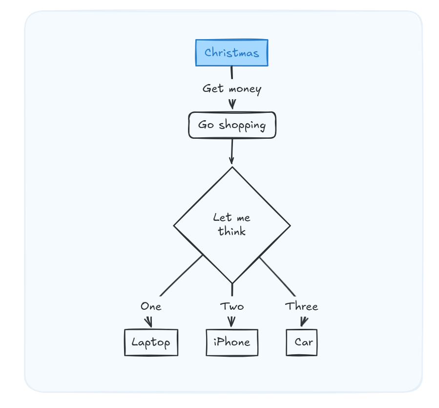
flowchart TD
    A[Christmas] -->|Get money|
    B(Go shopping)
    B --> C{Let me think}
    C -->|One| D[Laptop]
    C -->|Two| E[iPhone]
    C -->|Three| F[fa:fa-car Car]
Create the diagram’s Mermaid code assisted by AI, then …
Just paste MermaidJS into excalidraw instead and create awsome diagrams!
The trick also works from excel tables
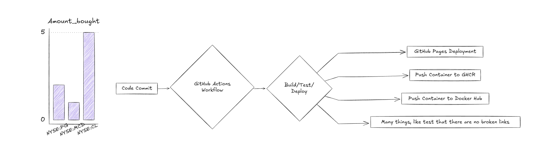
 Job Trends RepoCV-lAItex Repo
FAQ
PK vs SK for DWH
This is a fundamental concept in data modeling that separates transaction processing (OLTP) thinking from data warehousing/BI (OLAP) thinking.
In a Senior BI interview, you don’t just want to define them; you want to explain why the distinction is critical for a robust data warehouse.
1. The Primary Key (The General Concept)
A Primary Key (PK) is a broad database concept. It is a column (or a combination of columns) that uniquely identifies every single row in a table.
- Rule 1: It must be unique (no two rows can share the same PK).
- Rule 2: It cannot be null (empty).
In the real world, primary keys usually fall into two categories:
A. Natural Keys (Business Keys)
These are identifiers that exist in the real world outside of your data warehouse. They have business meaning.
- Examples: Social Security Number, Email Address, Vehicle Identification Number (VIN), ISBN for a book, or the
CustomerIDgenerated by your company’s Salesforce CRM (e.g., “CUST-NY-12345”).
B. Artificial Keys
These are keys created solely for the database because no good natural key exists.
- Examples: An auto-incrementing integer (1, 2, 3…) in a small application database, or a GUID/UUID.
2. The Surrogate Key (The BI Specialist)
A Surrogate Key (SK) is a specific type of artificial primary key used almost exclusively in dimensional modeling (data warehousing).
It is an integer (usually sequential: 1, 2, 3, 4…) that is generated by the ETL process or the data warehouse database itself as data is loaded into a dimension table.
Crucial Characteristics of a Surrogate Key:
- Zero Business Meaning: It is just a number. Business users should never see it or use it in a report.
- Owned by the Data Warehouse: It does not exist in the source system. The data warehouse controls its lifecycle completely.
- The “True” Primary Key of a Dimension: In a Kimball Star Schema, the surrogate key is always the primary key of a dimension table.
3. Comparison: Why do we need Surrogate Keys if we have Natural Keys?
This is the core of the interview answer. Why not just use the CustomerID from Salesforce as the primary key in your Data Warehouse Customer Dimension?
Here are the critical reasons why a Senior Architect insists on using Surrogate Keys instead of Natural Keys in a data warehouse:
A. Decoupling from Source Systems (Independence)
- Natural Key Problem: What happens if your company buys another company? Suddenly you have two different CRM systems. Company A has Customer ID “123” and Company B also has Customer ID “123”, but they are different people. If you used natural keys, your data warehouse breaks due to duplicate keys.
- Surrogate Key Solution: The ETL process assigns Company A’s customer SK
1and Company B’s customer SK2. The data warehouse doesn’t care that their source IDs are identical because it manages its own unique keys.
B. Performance (Join Speed)
- Natural Key Problem: Natural keys are often alphanumeric strings (e.g., “CUST-A-998-X”). Joining fact tables to dimension tables on long text strings is slow for database engines.
- Surrogate Key Solution: Surrogate keys are simple integers. Joining tables based on integers is the fastest operation a database can perform. In a 10-billion-row fact table, this difference is massive.
C. Handling History (SCD Type 2) - The most important reason
- Natural Key Problem: Natural keys identify a business entity (John Smith). If John Smith moves from New York to California, his business key (
CustomerID: JS123) doesn’t change. You cannot have two rows in your dimension table with the Primary KeyJS123. Therefore, you cannot track his history; you can only overwrite his address. - Surrogate Key Solution: Surrogate keys identify a specific version of a business entity at a point in time.
Example of SCD Type 2 enabled by Surrogate Keys:
| Surrogate Key (PK) | Natural Key (Business ID) | Customer Name | City | Is Current? |
|---|---|---|---|---|
| 101 | JS123 | John Smith | New York | False |
| 205 | JS123 | John Smith | California | True |
We now have two rows for the same business entity (JS123). This is only possible because the Primary Key of the table is the Surrogate Key (101 and 205), which are unique.
Summary Table for Interview
| Feature | Primary Key (Natural / Business Key) | Surrogate Key |
|---|---|---|
| Origin | Source System (CRM, ERP, Real World) | Generated by Data Warehouse ETL |
| Meaning | Has business meaning (e.g., SSN, Email) | Zero business meaning (just a number) |
| Data Type | Often alphanumeric text, GUIDs | Almost always Integer/BigInt |
| Join Performance | Slower (if text) | Fastest possible |
| Stability | Can change (rarely, but it happens) | Never changes once assigned |
| Primary Role | Uniquely identifies a business entity | Uniquely identifies a row in a dimension (enabling history) |
BI with AI?
If you dont want to Vibe code your own PoC with Streamlit…

You have some AI.BI Tools, like:
MIT | 🪄 Create rich visualizations with AI
- You can also vibe code a Python scripts to write for you tedious and repetitive Grafana dashboards (like the ~ x400 pannel creation)
Organizational Tools
You might need to do proper note taking for your KB.
Stay in touch and communicate with your colleagues.
For PMs in need of a who does what, there are several tools for them.
And Im not just talking about Jira/ADO.
Remember that ppts can be done via code, like so. With live data capabilities via API queries.
And also those pdf reports or the
For the db alergic ones, see:
CV Tools
I have been using a lot of resume templates.
From word, to pptx and later I explored canva, which resulting pdf had some parsing issues for some organizations.
Then, I switched gears to cv as a code approach: with OSS CV builders and with Latex via overleaf
- YAMLResume - This is the last I tried
Reactive Resume
Open Resume, which I forked here with a CI/CD powered Container
- Cool Latex CV Templates for Overleaf
And as some point I saw clear the setup: scrap offer + customize the cv code with LLMs as per your experience context, aka historieta: