FEM and a Self-Optimizing design loop
Tl;DR
In the MBSD series we asked where does each part go and how fast.
FEM asks what happens to the material when it gets there.
Same bodies, different question — motion becomes deformation.
Intro
Every post in the MBSD series treated mechanical bodies as rigid: a crank doesn’t bend, a connecting rod doesn’t stretch, a suspension wishbone doesn’t flex.
That assumption is what makes the equations of motion tractable — you get a clean ODE system for generalised coordinates $q(t)$ and integrate forward in time.
But real parts do deform. The cyclic loading from a firing I4 engine (see the engine NVH post) subjects the crankshaft to millions of bending and torsion cycles. The question MBSD cannot answer is: what does that do to the material? That is the domain of Finite Element Analysis.
From Motion to Deformation
Will the mechanisms designed as per the mbsd framework break in their operations?
The Rigid Body Assumption (and When It Breaks)
In every MBSD model, each body has a fixed mass $m$ and inertia tensor $\mathbf{I}$.
Forces produce accelerations.
The body moves as a whole — its shape never changes.
This is valid as long as structural deformations are small compared to the motion itself, which is true for most kinematic and dynamic analyses.
FEM drops that assumption.
A body is no longer a point mass or a rigid solid — it is a continuous elastic medium.
The goal shifts from integrating trajectories to finding a displacement field $\mathbf{u}(\mathbf{x})$: at every point in the solid, how much does the material move under load?
The Core FEM Equation
Where MBSD gives you:
$$\mathbf{M}\ddot{q} + \mathbf{C}\dot{q} + \mathbf{K}q = \mathbf{F}(t)$$
FEM (in its static structural form) gives you:
$$\mathbf{K},\mathbf{u} = \mathbf{F}$$
The stiffness matrix $\mathbf{K}$ encodes the material and geometry of the part. $\mathbf{F}$ is the applied load vector. $\mathbf{u}$ is the displacement at every node of the mesh — the answer you are looking for.
From $\mathbf{u}$ you derive strain $\boldsymbol{\varepsilon}$ (how much the material stretches) and stress $\boldsymbol{\sigma}$ (the internal force per unit area), connected by the material’s constitutive law:
$$\boldsymbol{\sigma} = \mathbf{C},\boldsymbol{\varepsilon}$$
where $\mathbf{C}$ is the elasticity tensor (for isotropic materials it collapses to just Young’s modulus $E$ and Poisson’s ratio $\nu$).
How the Mesh Works
FEM discretises the continuous domain into small elements — triangles and quads in 2D, tetrahedra and hexahedra in 3D. Over each element, the displacement is approximated by shape functions $N_i(\mathbf{x})$ that interpolate between nodal values.
The element stiffness matrix $\mathbf{k}_e$ is computed by integrating over the element volume:
$$\mathbf{k}e = \int{V_e} \mathbf{B}^T \mathbf{C}, \mathbf{B}, dV$$
where $\mathbf{B}$ is the strain-displacement matrix (derivatives of the shape functions).
Global $\mathbf{K}$ is assembled by summing all element contributions — same idea as assembling the global mass matrix in a rigid-body model.
The Link Back to the MBSD Series
The two methods are not alternatives — they are sequential in a real design loop:
- MBSD → compute the dynamic loads at each joint over the operating cycle (e.g. peak crank bearing force at 6000 rpm from the I4 model)
- FEM → apply those loads to the part geometry, find where stress concentrations appear
- Optimise → reshape the geometry to move stress peaks, reduce mass, or extend fatigue life
- Repeat → the updated geometry changes the inertia, so you go back to step 1
This is the self-optimising design loop in the post title. MBSD provides the boundary conditions; FEM evaluates the structure under them.
The dimensional reduction idea from the MBSD series still applies here: a 2D plane-stress FEM on a crank cross-section is fast and informative before committing to a full 3D solid mesh.
Conclusions
MBSD tells you how parts move. FEM tells you whether they survive the trip.
#git clone https://github.com/JAlcocerT/3Design
#freecad
exec(open("/home/jalcocert/Desktop/3Design/z-freecad/slider_crank_fem.py").read())
Writing time CalculiX input file: 0.006 seconds.
CalculiX solver run...
CalculiX finished without error.
CalculiX read results...
Read ccx results from frd file: /tmp/fcfem_joytblqk/FEMMeshGmsh.frd
Read ccx results from dat file: /tmp/fcfem_joytblqk/FEMMeshGmsh.dat
Solver: True
── FEM Results ──────────────────────────────────
Motor torque: 10.0 Nm
Crank length: 100 mm
Applied pin force: 100.0 N
Material: AlMgSi1F31
Max von Mises: 2.9595 MPa
Mean von Mises: 0.6178 MPa
Yield strength: 276 MPa (Al 6061-T6)
Safety factor: 93.26
OK — passes static check.
Max displacement: 0.0067 mm
─────────────────────────────────────────────────
Running them in sequence — loads from dynamics, stress from FEM, geometry update, repeat — is what the self-optimising loop in the title actually means.
FAQ
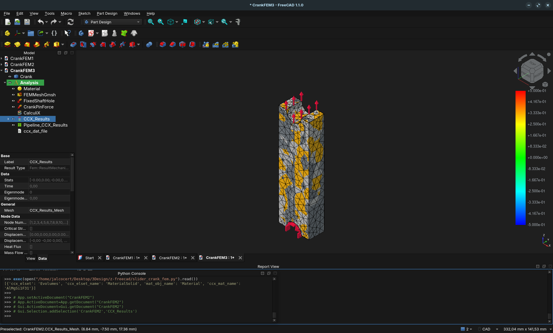
Can FreeCAD do this?
Yes. FreeCAD’s FEM Workbench is a fully capable GUI-driven FEM environment at no cost:
- Solver backend: CalculiX for structural and thermal analysis; Elmer for multiphysics (electromagnetics, fluid-structure interaction)
- Meshing: Gmsh or Netgen built in — you define the geometry in FreeCAD’s Part/PartDesign workbench and mesh it directly
- Workflow: import a STEP file (e.g. from CadQuery), assign material properties, apply boundary conditions (fixed face, force, pressure), run, and visualise stress/displacement contours
For the MBSD design loop this means: export the crank geometry from CadQuery → open in FreeCAD FEM → apply the peak bearing loads from the MBSD model → read off the von Mises stress map.
The CfdOF add-on adds CFD (via OpenFOAM) to the same geometry, so you can do both structural and flow analysis from one tool.
OSS Programs and Python Libraries for FEM
GUI / standalone solvers:
| Tool | What it does | Notes |
|---|---|---|
| FreeCAD FEM | Structural + thermal FEM via CalculiX / Elmer | Best GUI entry point; free |
| Elmer FEM | Multiphysics solver (structural, EM, FSI) | Finnish government-backed; own GUI |
| CalculiX | Structural FEM, Abaqus-compatible input | No GUI, but FreeCAD wraps it |
| Code_Aster | Large-scale structural/thermo-mechanical | Used by EDF; very mature |
| Salome-Meca | GUI front-end for Code_Aster | Ships together as a bundle |
Python libraries:
The Heavyweights (Research and Multiphysics)
For solving complex PDEs — structural stress, heat dissipation, electromagnetics:
- FEniCS / FEniCSx — write the weak form of your physics in Python using UFL; it generates optimised C++ under the hood. Best for custom physics and HPC.
- Firedrake — same UFL input language as FEniCS, different parallel backend. Excellent for unstructured tetrahedral meshes.
- SfePy — batteries-included: pre-built solvers for fluid-structure interaction, heat conduction, acoustics. Less setup than FEniCS.
Specialised for Engineering
- Akantu — C++ core with a Python interface; designed for solid mechanics, contact, and fracture.
- CALFEM for Python — port of the Lund University MATLAB toolkit. Transparent and educational; ideal if you want to see every matrix assembly step.
- PyFEA — lightweight 2D/3D structural analysis; good for quick parametric studies.
The Full Pipeline (CAD → Mesh → Solve → Visualise)
| Step | Tool |
|---|---|
| Geometry (CAD) | CadQuery (Python) or FreeCAD |
| Meshing | Gmsh + gmsh-sdk Python API |
| Solving | FEniCS, SfePy, or CalculiX |
| Visualisation | PyVista (VTK wrapper) or ParaView |
Which one should you pick?
| If you want… | Use this |
|---|---|
| To learn FEM from scratch | CALFEM |
| GUI with no coding | FreeCAD FEM Workbench |
| Custom PDEs / research | FEniCS / Firedrake |
| Ready-to-go structural solvers | SfePy or Akantu |
| Interactive 3D results in Python | PyVista |
A Minimal FEM Example in Pure Python
The following assembles the global stiffness matrix $\mathbf{K}$ and solves $\mathbf{K}\mathbf{u} = \mathbf{F}$ for a simple two-element bar — the same matrix equation from the theory section, made concrete with numpy:
import numpy as np

# Two-element bar: 3 nodes, fixed at node 0, 10 kN load at node 2
# Steel: E = 200 GPa, cross-section A = 1e-4 m^2, element length L = 0.5 m
E, A, L = 200e9, 1e-4, 0.5
k = E * A / L  # element axial stiffness

# Assemble global stiffness matrix (3x3)
K = np.array([
    [ k, -k,  0],
    [-k, 2*k, -k],
    [ 0, -k,  k]
])

# Apply BC: node 0 fixed (u0 = 0) — reduce system to free DOFs
K_free = K[1:, 1:]
F_free = np.array([0.0, 10e3])  # 10 kN at node 2

# Solve
u_free = np.linalg.solve(K_free, F_free)
u = np.array([0.0, *u_free])

# Recover stress in each element: σ = E · ε = E · Δu / L
sigma = [E * (u[i+1] - u[i]) / L for i in range(2)]

print(f"Displacements: {u * 1e3} mm")
print(f"Stress element 1: {sigma[0]/1e6:.1f} MPa")
print(f"Stress element 2: {sigma[1]/1e6:.1f} MPa")
This is the same $\mathbf{K}\mathbf{u} = \mathbf{F}$ the theory describes, assembled by hand. Real FEM libraries do the same thing — just for thousands of elements in 3D, with shape functions handling the geometry automatically.