MBSD 2D. Flat > Boxer?
Tl;DR
After the ,failed’ I4 attempt it goes…
Intro
All Boxer are flat 180, but not viceversa.
flat are v at 180 degrees that share crank pin, but boxer have different crank pins
MBSD 2D x Vibrations
Trying to make a quick bypass with LLMs was not a good idea here.
So I upgraded the mbsd framework to make such kind of analysis.
About Vibrations, FTT and NVH
Dominant harmonic content (for any slider-crank at constant ω):
- 1st harmonic (once per rev) — gravity + translating-mass imbalance
- 2nd harmonic (twice per rev) — the famous “secondary” inertia force, caused by the finite rod length (R/L term in the acceleration expansion). This is exactly why 4-cylinder engines need balance shafts
How come, FFTs again when jumping to the frequency domain.
One Slider Crank + Gravity
Slider Crank No Gravity
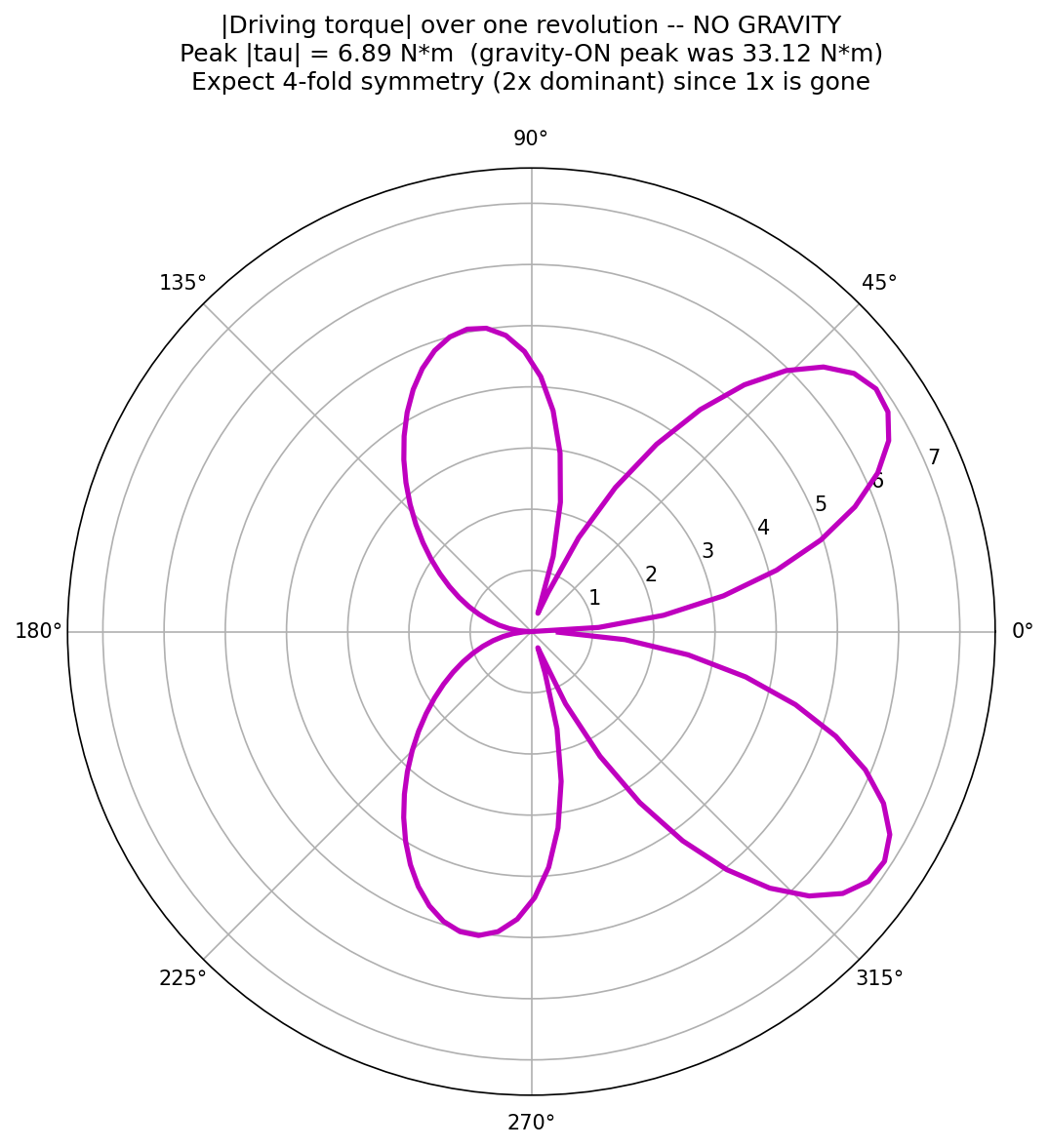
Engine Configuration vs Vibrations
Im getting away with the 2D implementation so far :)
Flat 4
Boxer 4
Every boxer is a flat 4, but not every flat 4 is a boxer.
Flat vs Boxer
The distinction lies entirely in the crankshaft throws, and you can break it down using the logic you’ve built in your series:
- The Shared Geometry (The “Flat” part)
Both engines are horizontally opposed.
They both use the bank-mirror sign pattern $[+1, -1, +1, -1]$ because the pistons physically move in opposite directions in world coordinates.
This is why both cancel their net forces ($F = 0$) at every harmonic.
- The Crankshaft (The “Boxer” part)
The defining characteristic of a Boxer is that each cylinder has its own dedicated crankpin, and opposed pairs are phased $180^\circ$ apart relative to each other.
- Result: Opposed pistons reach Top Dead Centre (TDC) at the same time. They “box” toward and away from each other.
- Phasor Sum: The kinematic phases for an opposed pair are the same (e.g., $0^\circ$ and $0^\circ$). Because the sign flip is applied, they cancel immediately: $1 - 1 = 0$.
- The Non-Boxer (The “180° V” or “Flat” engine)
In a non-boxer flat engine (like the one used in some Ferraris or the Lancia Fulvia), opposed pistons often share a crankpin or use an Inline-4 style crank.
- Result: When one piston is at TDC, its opposite partner is at Bottom Dead Centre (BDC). They move in the same world direction at the same time (e.g., both moving “Left” together).
- Phasor Sum: The kinematic phases for an opposed pair are $180^\circ$ apart (e.g., $0^\circ$ and $180^\circ$).
- Cylinder 1: $+1 \cdot \exp(j \cdot 0^\circ) = +1$
- Cylinder 2: $-1 \cdot \exp(j \cdot 180^\circ) = -1 \cdot (-1) = +1$
- Net effect: They reinforce each other’s momentum in the short term, leading to the 1× rocking couple you just analyzed.
The Final Classification
- Boxer-4: A subset of flat-4s where the crankpins are arranged so that opposed pistons are in phase ($s_1\phi_1 + s_2\phi_2 = 0$). Balanced in force AND moment.
- Non-Boxer Flat-4: A flat-4 where the crankpins are arranged like an I4 ($180^\circ$ apart). Balanced in force, but unbalanced in moment.
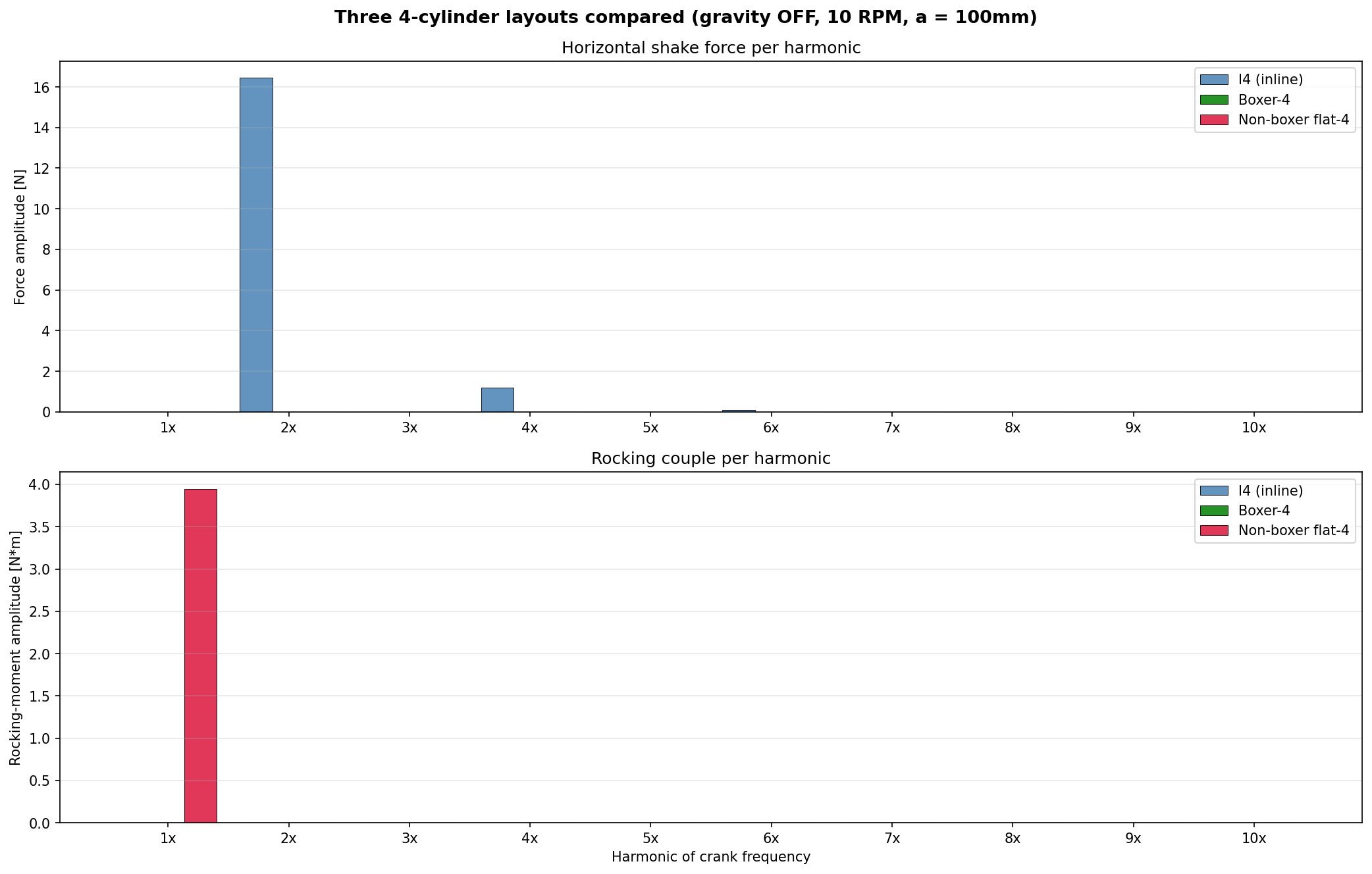
| Layout | Force 1× | Force 2× | Moment 1× | Moment 2× |
|---|---|---|---|---|
| I4 (inline) | 0 | 16.44 N | 0 | 0 |
| Boxer-4 | 0 | 0 | 0 | 0 |
| Non-boxer flat-4 | 0 | 0 | 3.95 N·m | 0 |
Proper I4 Analysis
I wont let you with the ai slop previous analysis.
# Default: 10 RPM, R=1, L=2
python 2D-Dynamics/examples/multi-cylinder-nograv/engine_comparison.py

# Custom R/L
python -c "import engine_comparison as e; e.main(rpm=10, R=0.8, L=3.0)"

# R/L sweep
python -c "import engine_comparison as e; e.sweep_RL(R=1.0, L_values=[1.5, 2.0, 3.0, 4.0])"
This data is the “smoking gun” for engine balance theory.
By isolating the forces and moments at these specific toy parameters, you’ve created a perfect fingerprint for each layout.
- The Zero-Force Rule: Notice that every engine on your list except the I4 has
(none)for force.
This confirms that 3, 4, and 6-cylinder layouts are generally excellent at cancelling Primary (1×) and Secondary (2×) linear shake—the I4 is the famous outlier because its $2\times$ secondary phasors all point in the same direction.
- The Rocking Rivalry: Comparing the Straight-3 ($1.71\text{ N}\cdot\text{m}$) to the Non-boxer flat-4 ($3.95\text{ N}\cdot\text{m}$) is eye-opening.
Even though the flat-4 has more cylinders and cancels its force, its rocking couple is 2.3 times more violent than the notoriously “thrummy” three-cylinder.
This is the mathematical reason why the non-boxer flat-4 is a historical rarity.
- The Gold Standards: The Boxer-4 and Straight-6 both hitting
(0, 0)is the verification of the “Inherently Balanced” title.
One achieves it through mirror-image pairs (sign-flip), the other through $120^\circ$ symmetry (phasor-sum).
| Configuration | The “Vibe” | The Physics |
|---|---|---|
| Straight-3 | Thrummy / Rocking | $1\times$ force cancels, but the lever arms create a seesaw moment. |
| Inline-4 | High-frequency Buzz | Perfect primary balance, but $2\times$ secondary forces stack linearly. |
| Boxer-4 | Stillness | Opposed cylinders share the same phase; sign-flip kills every harmonic. |
| Non-boxer flat-4 | Heavy Pitching | I4 phasing in a flat layout turns the $2\times$ shake into a $1\times$ rock. |
| Straight-6 | Turbine-like | Forces and moments cancel at $1\times$ and $2\times$ by pure geometry. |
A Quick Sanity Check
Looking at your I4 Force (16.44 N): Since $F_{2\times} \approx 4 \cdot F_{single} \cdot (R/L)$, and your $R/L$ is $0.5$, this implies your single-cylinder secondary force is roughly $8.22\text{ N}$ at these parameters.
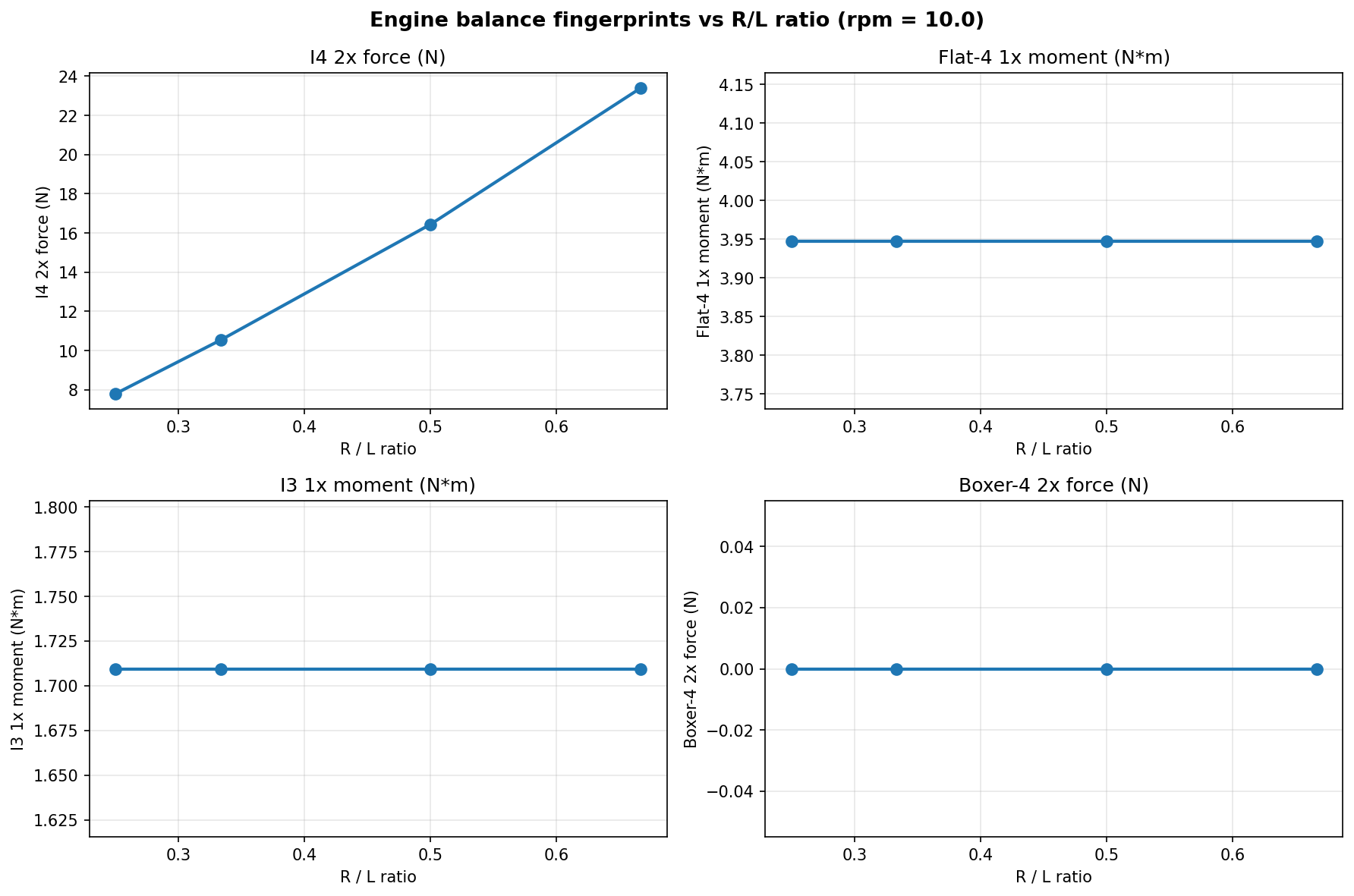
Why does 2× scale with R/L but 1× doesn’t?
Taylor-expands L·√(1 − (R/L)²·sin²θ) using sin²θ = (1 − cos 2θ)/2 to show that piston acceleration has a 1× term (ω²·R — no L dependence) and a 2× term (ω²·R²/L = ω²·R·(R/L)).
Ends with the engineering consequence: longer rods reduce secondary imbalance linearly, production I4s hit the R/L ≈ 0.25–0.33 wall and then need balance shafts.
Conclusions
I was not happy with the quick engine-balance concept and this has been the fix.
This has been a good excuse to test opus 4.7 via the CC Max plan:

Have you noticed the gap of value from such subscription from the similarly priced today accounting ones?
What am i talking about…
Beyond food and warm, what do you like?
 Consulting Services
 DIY via ebooks
FAQ
What are those concepts?
The Saddle-Point System is the mathematical engine under the hood of most professional multibody dynamics solvers.
It is a specific structure of linear equations that arises whenever you need to solve for motion subject to constraints—like a piston head that is forced to stay within a cylinder.
In our project, this system allows us to solve for both the accelerations of the parts and the reaction forces at the joints simultaneously.
The Matrix Structure
The system is organized into a block matrix that looks like this:
$$\begin{bmatrix} M & C_q^T \ C_q & 0 \end{bmatrix} \begin{bmatrix} a \ \lambda \end{bmatrix} = \begin{bmatrix} Q_{total} \ \gamma \end{bmatrix}$$
- $M$ (Mass Matrix): This top-left block contains the masses and moments of inertia for all bodies in the system.
- $C_q$ (Constraint Jacobian): This represents the “geometry of the joints.” It defines how the coordinates are locked together.
- $a$ (Accelerations): The primary unknown. These are the linear and angular accelerations we need to integrate to find the next position.
- $\lambda$ (Lagrange Multipliers): These represent the constraint forces. In our analysis, this is where we extract $R_x$, $R_y$, and the driving torque $\tau$.
- The Zero Block: The bottom-right $0$ is the defining “saddle” feature. It exists because constraints don’t “push back” with their own mass; they only enforce geometric rules.
Why It Is Called a “Saddle Point”
The name comes from optimization theory.
If you view the engine as a system trying to minimize its energy while staying on the track of its constraints, the solution $(a, \lambda)$ is a minimum with respect to the accelerations but a maximum with respect to the constraint forces.
This creates a “saddle” shape in the mathematical landscape.
Application in the Series
- Forward Dynamics: We provide the forces ($Q_{total}$) and solve for $a$.
- Inverse Dynamics: We provide the motion ($a$ is known via constraints) and solve for the $\lambda$ values required to make that motion happen.
- Vibration Source: By solving this system at every time step, we generate a high-fidelity time-series of $\lambda(t)$. When we feed those multipliers into an FFT, we get the vibration spectrum that identifies the “I4 buzz” or the “Subaru hum.”
Holonomic vs Non Holonomic Constrains
A holonomic constraint is an equation of the form
$$C(q, t) = 0$$
“Holonomic” means it depends only on positions (and possibly explicit time), not on velocities.
Expanding into non-holonomic constraints moves the physics from “geometry of position” to “geometry of motion.”
While holonomic constraints reduce the space of where a body can be, non-holonomic constraints restrict how a body can move between those positions.
1. The Definition: Velocity Dependence
A non-holonomic constraint is typically expressed at the velocity level and cannot be integrated back into a position-only equation. It takes the form:
$$C(q, \dot{q}, t) = 0$$
Unlike a slider-crank joint (where if you know the crank angle, you know the piston position), a non-holonomic system’s position depends on the path taken, not just the current state.
2. Classic Example: The Rolling Disk (Knife-Edge)
Imagine a vertical coin rolling on a plane without slipping.
- Holonomic part: The coin stays on the ground ($y = R$).
- Non-holonomic part: The coin must move in the direction it is pointing.
If the coin’s orientation is $\theta$ and its position is $(x, z)$, the velocity constraint is:
$$\dot{x} \sin \theta - \dot{z} \cos \theta = 0$$
You cannot turn this into an equation like $f(x, z, \theta) = 0$. If you could, you would be saying the coin is trapped on a specific curve on the floor.
Instead, by rolling and steering, the coin can eventually reach any $(x, z)$ position on the floor, but it can’t move sideways instantly.
3. Implications for the “Computational Machinery”
Adding non-holonomic constraints to your solver changes the math in three significant ways:
A. Degrees of Freedom Paradox
In a holonomic system, $DOF = \text{coordinates} - \text{constraints}$. In a non-holonomic system, you have a split:
- Kinematic DOFs: The number of independent velocities you can choose (restricted).
- Configuration DOFs: The number of coordinates needed to describe the position (unrestricted).
A car has 2 kinematic DOFs (gas and steer) but 3 configuration DOFs (it can reach any $x, y, \theta$ in a parking lot).
B. The Saddle-Point System Update
Your saddle-point matrix still works, but the $\gamma$ term and the Jacobian change. For a velocity constraint $A(q)\dot{q} = 0$, the acceleration-level constraint becomes:
$$A(q)\ddot{q} + \dot{A}(q, \dot{q})\dot{q} = 0$$
The Lagrange multipliers ($\lambda$) now represent the forces of constraint required to prevent slipping or sideways sliding (e.g., the lateral friction of a tire).
C. Path Dependency (The “Parallel Parking” Effect)
Because you can’t integrate these constraints to find a position, you cannot use a simple Newton-Raphson position solver to find a valid state.
You must integrate the velocities over time to know where the system ended up.
This makes “Inverse Kinematics” for non-holonomic systems (like autonomous driving) much harder than for a simple robotic arm.
| Feature | Holonomic | Non-Holonomic |
|---|---|---|
| Equation Type | $C(q, t) = 0$ | $C(q, \dot{q}, t) = 0$ |
| Integrability | Integrable to positions | Not integrable |
| Constraint Focus | Restricts “where” you can be | Restricts “how” you can move |
| Example | Revolute joint, gear pair | Rolling wheel, ice skate, sled |
| Solver Impact | Reduces coordinate space | Restricts velocity space only |
Does your current simulator need to handle “pure rolling” for the vehicle examples, or are you sticking to the “penalty-friction” approach which mimics non-holonomic behavior without the hard algebraic constraint?