Fluidssss
TL;DR
How about bringing fluid mechanics to the ICEs?
+++ migrated to py the good old matlab MCIA model
Intro
A constant speed at an ICE crank?
What kind of model was that?
Reality is: intermitent forces driven by combustions are the ones pushing the slider down!
About Fluid Mechanics
Bernuli
The Missing Half of the MBSD Picture
Every engine post in the MBSD series treated the combustion force as a known input — a prescribed pressure pushing the piston down at the right moment.
That is a clean assumption for studying crankshaft balance and NVH, but it hides the question: where does that force actually come from?
The answer is fluid mechanics.
Specifically, the thermodynamics of a gas being compressed and then ignited.
Fluid mechanics is the discipline that lets you compute $P(\theta)$ — the cylinder pressure as a function of crank angle — rather than just assuming it.
The conceptual shift mirrors the one from MBSD to FEM:
| Discipline | Question | Solves for |
|---|---|---|
| MBSD | How do bodies move under given forces? | $q(t)$, $\dot{q}(t)$ — positions and velocities |
| FEM | How does material deform under given loads? | $\mathbf{u}(\mathbf{x})$ — displacement field |
| Fluid Mechanics | Where do those forces come from? | $P$, $\rho$, $T$, $\mathbf{v}$ — pressure, density, temperature, velocity |
The Governing Equations
Fluid mechanics is built on three conservation laws applied to a continuous medium:
1. Conservation of mass (continuity):
$$\frac{\partial \rho}{\partial t} + \nabla \cdot (\rho \mathbf{v}) = 0$$
What goes in must come out — mass cannot appear or disappear inside a control volume.
2. Conservation of momentum (Navier-Stokes):
$$\rho \left(\frac{\partial \mathbf{v}}{\partial t} + \mathbf{v} \cdot \nabla \mathbf{v}\right) = -\nabla P + \mu \nabla^2 \mathbf{v} + \mathbf{f}$$
Forces on a fluid element — pressure gradients, viscosity, and body forces — produce acceleration. This is Newton’s second law for fluids.
3. Conservation of energy:
$$\rho c_v \frac{DT}{Dt} = -P,(\nabla \cdot \mathbf{v}) + \nabla \cdot (k \nabla T) + \dot{q}_{combustion}$$
Temperature changes come from compression work, heat conduction, and heat release from combustion.
For an ideal gas these three equations are closed by the equation of state:
$$P = \rho R T$$
For an ICE: From Crank Angle to Cylinder Pressure
Inside a cylinder, the volume changes with crank angle $\theta$ following the slider-crank geometry (which you already know from the MBSD posts).
- https://github.com/JAlcocerT/mbsd/blob/master/z-fluid-mechanics/dinamica-gases-py.md
- https://github.com/JAlcocerT/mbsd/blob/master/z-destilled-ebook/2d-slidercrank-multicylinder-combustion.md
Assuming an ideal Otto cycle, the pressure during the compression and expansion strokes follows a polytropic process:
$$P V^\gamma = \text{const}$$
where $\gamma = c_p / c_v \approx 1.35$ for hot combustion gases. This gives you the pressure trace $P(\theta)$ that acts on the piston crown — the force input that the MBSD engine models take as given.
The combustion event itself adds a spike on top: the heat release from burning fuel raises temperature almost instantaneously at TDC, which via the ideal gas law drives a sharp pressure rise.
Integrating $P(\theta)$ over the piston area and projecting along the connecting rod gives you exactly the slider force that feeds into the dynamics.
This is the loop: fluid mechanics computes the gas forces → MBSD propagates them through the mechanism → FEM checks whether the parts survive the resulting stress.
Application of Gas mechanics
The ICE!
It was a very interesting time back then.
I mean…when I was doing this kind of things in matlab.
But similarly as I did with the bike simulator, it is time to bring them to python.
Isnt it nice to see the volumetric efficiency interactively?
Conclusions
Im still amazed at people like FarmCraft101 and their subs who provide OSS cad design for a new turbine which x2 the energy collection:
Crazy….
This is being the year of bridging concepts.
I would have never guessed how, where and when I would be coming back to them.
The executing speed is less of a problem nowadays
The blocker is being more about knowledge management.
For that, you can always:
 Consulting Services
 DIY via ebooks
FAQ
Volumetric efficiency
One of the best videos to understand VE:
You can also make an engineering BSc and port your matlab files to explore more:
git clone /mbsd
cd ./mbsd/z-fluid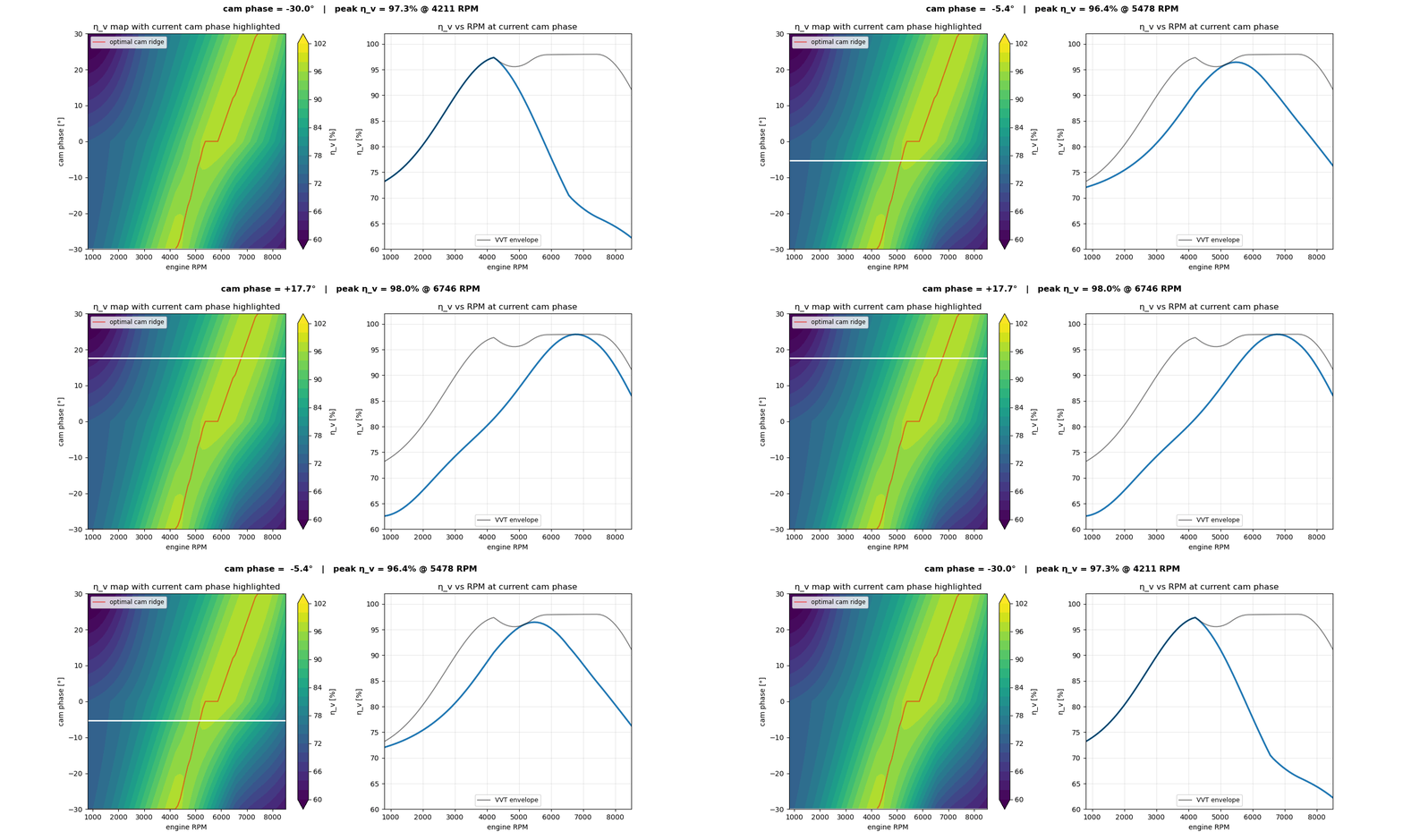
Volumetric efficiency ($\eta_v$) measures how well an engine breathes — how much fresh charge actually enters the cylinder compared to what could theoretically fit:
$$\eta_v = \frac{m_{actual}}{m_{ideal}} = \frac{\text{mass of air-fuel charge inducted}}{\rho_{ambient} \cdot V_{displacement}}$$
A naturally aspirated engine at peak torque typically reaches $\eta_v \approx 85\text{–}95%$.
The gap from 100% comes from several fluid-mechanical losses:
| Loss source | Mechanism | Effect on $\eta_v$ |
|---|---|---|
| Intake restriction | Throttle, filter, port — pressure drop reduces charge density | $-5$ to $-15%$ |
| Residual gases | Hot exhaust gases left in clearance volume displace fresh charge | $-5$ to $-10%$ |
| Charge heating | Intake port and valve heat the incoming air, reducing density | $-3$ to $-8%$ |
| Late intake valve closing | At high RPM, inertia can ram extra charge in (beneficial) or cause backflow (harmful) | $\pm$variable |
| Valve curtain area | Flow is choked by the annular gap at the valve seat | RPM-dependent |
The VE–RPM Curve
VE is not a fixed number — it varies with engine speed, and its shape is what engine tuners care about:
- At low RPM: slow piston velocity means low charge inertia; the intake valve closes before the cylinder is full → low VE
- At peak torque RPM: intake runner length is tuned so pressure waves arrive just before valve closing, ram-charging the cylinder → peak VE
- At high RPM: flow velocity through the valves approaches sonic limits; viscous and inertia losses dominate → VE drops
This is why intake runner length is tuned for a target RPM band.
Short runners favour high-RPM power; long runners favour mid-range torque.
Variable-length intake manifolds (Honda VTEC, BMW Valvetronic, Toyota VVTL-i) shift the VE peak across the rev range.
VE Map
In engine management, VE is stored as a 2D lookup table (map) indexed by RPM and throttle position (or manifold pressure).
The ECU multiplies the map value by ambient air density to compute the injected fuel mass — this is the basis of speed-density fuelling:
$$m_{fuel} = \frac{\eta_v \cdot \rho_{air} \cdot V_{disp} \cdot n}{2 \cdot \lambda \cdot AFR_{stoich}}$$
where $n$ is engine speed (rev/s), the factor of 2 accounts for the 4-stroke cycle, $\lambda$ is the air excess ratio, and $AFR_{stoich}$ is the stoichiometric air-fuel ratio (~14.7 for petrol).
A VE map measured on a dyno (or estimated from pressure-trace data) is exactly the kind of table that feeds into the 0D combustion model from the heat transfer post — it sets the initial charge mass, which determines peak pressure and therefore the combustion force on the piston crown.
VE map reference: Tactrix open-source ECU data
The Analogy
Heat can be related to electro-magnetism, remember?
We can bring fluid variables to that same play:
In fact, the “Triple Analogy” between Electricity, Heat, and Fluid Mechanics is one of the most elegant corners of physics.
When you combine them, you get what engineers call Lumped Element Modeling.
Just as we mapped heat to electricity, we can map fluid flow to both.
The “Master Variable” in fluid mechanics that corresponds to Voltage or Temperature is Pressure.
- The Fluid-Electric-Thermal Mapping
If you can visualize water flowing through a pipe, you can understand a circuit or a heat exchanger.
| Electrical | Thermal | Fluid Mechanics |
|---|---|---|
| Voltage ($V$) | Temperature ($T$) | Pressure ($P$) |
| Current ($I$) | Heat Flow ($q$) | Volumetric Flow Rate ($Q$) |
| Resistance ($R$) | Thermal Resistance ($R_{th}$) | Hydraulic Resistance ($R_h$) |
| Capacitance ($C$) | Thermal Mass ($C_{th}$) | Compliance / Tank Volume |
| Inductance ($L$) | (No direct simple analog) | Inertance (Fluid Mass/Inertia) |
- How Fluid Components “Mimic” the Others
Hydraulic Resistance (The Pipe)
A narrow pipe or a clogged filter acts exactly like a resistor.
- The Math: $\Delta P = Q \cdot R_h$ (This is essentially Ohm’s Law for fluids).
- The Physics: To push more water (Current) through a thin straw (High Resistance), you need to blow harder (Increase Pressure/Voltage).
Fluid Compliance (The Water Tower)
A large tank or an elastic balloon in a plumbing system acts like a capacitor.
- In Electricity: A capacitor stores charge and resists sudden changes in voltage.
- In Fluids: A water tower stores potential energy and keeps the city’s water pressure from dropping the second everyone turns on their taps.
It “smooths out” the pressure.
Fluid Inertance (The “Water Hammer”)
This is a unique fluid property that is the perfect analog for an Inductor ($L$) in a circuit.
- When you suddenly shut a faucet and hear a “thump” in the walls, that is Inductance.
The moving fluid has mass and “wants” to keep moving, just like an inductor resists a change in current.
Heat transfer doesn’t really have a natural version of this, which makes thermal systems much “simpler” (and more sluggish) than fluid or electric ones.
- The “Power” Connection
In all three systems, Power is calculated by multiplying the “Push” (Across variable) by the “Flow” (Through variable):
- Electric Power: $P = V \cdot I$
- Thermal Power: $P = \Delta T \cdot q$ (Though $q$ is already a power unit, Watts)
- Fluid Power: $P = \Delta P \cdot Q$
- Why this matters for Heat Transfer
In real engineering, these analogies often collide!
Think of a Liquid Cooling System in a high-end PC:
- The CPU creates “Current” (Heat).
- The Water acts as a “Carrier” (Fluid Flow).
- The Pump provides the “Voltage” (Pressure) to overcome the “Resistance” (Narrow tubes).
- The Radiator acts as a “Transformer,” transferring the “Current” from the fluid system into the air.
The Limits of the Analogy
While the “math” matches up beautifully for Laminar Flow (smooth water), it breaks down once the fluid becomes Turbulent.
- In electricity, $V=IR$ is almost always a straight line (linear).
- In fluids, if you double the flow, the pressure required might quadruple (non-linear).
Tools
High-performance C++ library for multiphysics and multibody dynamics simulations
OpenModelica is an open-source Modelica-based modeling and simulation environment intended for industrial and academic usage.
OSS Programs and Python Libraries for Fluid Mechanics
Can FreeCAD do this?
FreeCAD has two relevant workbenches:
- FEM Workbench — structural and thermal FEM via CalculiX and Elmer solvers, with a GUI mesh generator. Good for static stress and simple heat transfer, not CFD.
- CfdOF Add-on — a CFD workbench built on top of OpenFOAM.
You define geometry in FreeCAD, mesh it (SnappyHexMesh or cfMesh), set boundary conditions, and run OpenFOAM in the background.
Visualisation is done via ParaView.
This is the closest you get to a free ANSYS Fluent workflow.
git clone /3Design
cd /z-openfoam
make all #make help
GUI / standalone solvers:
| Tool | What it does | Notes |
|---|---|---|
| OpenFOAM | General-purpose CFD (incompressible, compressible, reacting flow) | Industry standard OSS CFD; steep learning curve, powerful |
| SU2 | CFD + adjoint-based optimisation | From Stanford; good for aerodynamics and shape optimisation |
| Elmer FEM | Multiphysics including fluid-structure interaction | Finnish government-backed; GUI available |
| Code_Saturne | Turbulent industrial CFD | From EDF; handles complex geometries well |
| DWSIM | Chemical process simulation with thermodynamics | Good for ICE thermodynamic cycle modelling |
Python libraries:
| Library | Use case |
|---|---|
| Cantera | Combustion chemistry and thermodynamics — the right tool for computing the pressure trace $P(\theta)$ in an ICE from first principles |
| CoolProp | Thermophysical properties of real fluids (density, enthalpy, viscosity as functions of $P$ and $T$) |
| fluids | Engineering pipe flow, friction factors, fittings — Darcy-Weisbach and beyond |
| thermo | Equation-of-state thermodynamics for mixtures |
| PyFluids | Wrapper around CoolProp with a cleaner API |
| fipy | PDE solver that can handle the full Navier-Stokes if you want to write it yourself |
| pySPH | Smoothed Particle Hydrodynamics — mesh-free, good for free-surface flows |
For the ICE use case specifically, the practical Python stack is:
# pip install cantera coolprop fluids
import cantera as ct

# Define the gas mixture (air + fuel)
gas = ct.Solution('gri30.yaml')
gas.TPX = 300, 101325, 'CH4:1, O2:2, N2:7.52'

# Compress to TDC (polytropic)
gas.SP = gas.s, gas.P * (compression_ratio ** gamma)

# Ignite and get pressure
r = ct.IdealGasReactor(gas)
sim = ct.ReactorNet([r])
sim.advance(1e-3)
print(f"Peak pressure: {r.thermo.P/1e5:.1f} bar")
This gives you the combustion pressure that feeds directly into the MBSD slider-crank force model.
Betz’s Law and the Limits of Fluid Energy Extraction
The Betz Limit (formulated in 1919 by Albert Betz) is a fundamental result in fluid dynamics that establishes the maximum possible efficiency for any turbine operating in an open flow.
It is a clean example of how continuity and momentum conservation together impose a hard ceiling on what engineering can achieve.
What it states: no turbine can capture more than 59.3% of the kinetic energy in a flowing fluid.
The maximum power coefficient is:
$$C_p = \frac{16}{27} \approx 0.593$$
The reasoning is elegant.
If a turbine extracted 100% of the kinetic energy, the fluid downstream would be stationary — and stationary fluid cannot make room for incoming fluid, so the flow stalls.
If the turbine extracts nothing, the fluid passes through unchanged.
The optimum is somewhere in between: the fluid must leave with enough velocity to keep moving out of the way.
Solving the momentum balance across a rotor disk gives exactly $16/27$.
Why Hydro Turbines Are Not Bound by Betz
Betz Law applies specifically to open-flow systems — where the fluid can expand and divert around the rotor.
Most hydroelectric turbines operate in closed conduits, which changes the physics entirely:
Open vs. closed systems — in a pipe or casing, water cannot “escape” around the blades. Every kilogram of water must pass through the runner. This confinement allows pressure to do work that velocity alone cannot.
Pressure energy vs. kinetic energy — wind turbines extract kinetic energy from moving air. Hydro turbines mostly extract potential energy (head) converted to pressure. The Betz derivation does not apply to pressure-driven systems.
Incompressibility — water is ~800× denser than air and effectively incompressible. In a wind turbine the stream tube must widen as air slows down. In a pipe the cross-section is fixed, so flow diversion is not an issue.
The exception is hydrokinetic turbines (in open rivers or tidal streams without a dam).
These sit in open flow just like wind turbines and are subject to the same 59.3% limit.
The Three Classic Hydro Turbines
Each is engineered for a specific combination of head (pressure) and flow rate:
Pelton (Impulse)
Designed for high head, low flow — mountain streams falling hundreds of metres through a narrow pipe.
A nozzle converts pressure to a high-speed jet; the jet strikes spoon-shaped buckets at atmospheric pressure.
Energy is extracted purely through momentum change.
Because the water jet is concentrated and controlled, efficiencies above 90% are routine.
No open-flow diversion problem, hence no Betz limit.
Francis (Reaction)
The most common turbine in the world (Hoover Dam).
Designed for medium head and medium-to-high flow. Water enters radially through a spiral casing, passes through the runner blades, and exits axially.
It operates fully submerged and uses both velocity and pressure — the pressure drop across the blades “reacts” against them to produce torque.
Efficiencies up to 95%. Fully enclosed, so Betz does not apply.
Kaplan (Reaction / Propeller)
Essentially a large ducted propeller. Designed for low head and very high flow — large, slow-moving rivers.
Adjustable blades allow it to remain efficient as river levels change through the year.
Like the Francis it is a reaction turbine enclosed in a housing, forcing all flow through the runner.
Efficiencies typically 90–93%.
| Turbine | Type | Head | Flow | Best use case |
|---|---|---|---|---|
| Pelton | Impulse | High | Low | Mountain / alpine |
| Francis | Reaction | Medium | Medium–High | Large dams |
| Kaplan | Reaction | Low | Very high | Flat rivers, tidal |
The common thread: where a wind turbine must “let go” of some energy just to keep air moving away, these hydro designs control every drop through a closed path — which is why they all exceed the Betz limit comfortably.
Not with a 20-meter drop. While large Pelton turbines can exceed 90% mechanical efficiency under optimal conditions, a 20 m head is far too low for a Pelton wheel to run efficiently.
For a 20 m drop, a Pelton turbine will typically yield only 50% to 70% (or worse at small scales), whereas a Crossflow (Banki), Francis, or small Kaplan/propeller turbine is the proper choice to hit 80% to 88% efficiency.
Why a Pelton Wheel Fails at 20 Meters
Pelton wheels are impulse turbines designed for high head ($> 100\text{–}200\text{ m}$) and low flow.
Here is why low head ruins their performance:
- Sluggish Jet Velocity: A Pelton wheel converts the pressure head entirely into a high-speed jet via a nozzle:
$$v = \sqrt{2gh} = \sqrt{2 \times 9.81 \times 20} \approx 19.8\text{ m/s}$$
In high-head plants ($300\text{ m}$), jet speeds exceed $75\text{ m/s}$. At just $20\text{ m/s}$, the kinetic energy density of the jet is very low. 2. The Bucket-to-Wheel Ratio Problem: Optimal Pelton efficiency requires the wheel’s rim speed ($u$) to be roughly half the jet speed ($u \approx 0.46 \times v \approx 9.1\text{ m/s}$). To generate meaningful power with low head, you need a high volume of water ($Q$). A high flow rate requires a large nozzle diameter ($d$). However, a Pelton wheel only maintains high efficiency if the wheel diameter ($D$) is at least 10 to 15 times the nozzle diameter ($D/d \ge 10$). If $d$ is too wide relative to $D$, the jet splashes across the bucket edges, deflects unevenly, and chokes the casing, tanking efficiency. 3. Generator RPM Mismatch: If you make the wheel large enough to satisfy the $D/d$ ratio, a rim speed of $9.1\text{ m/s}$ translates to a very low rotational speed (e.g., 200–300 RPM). Standard electrical generators run at 1500 or 3000 RPM, forcing you to use a gearbox or belt drive—introducing mechanical friction losses of 5% to 15%.
What Turbine Should You Use for 20 Meters?
At $20\text{ m}$ (classified as medium-to-low head), the selection depends on your water flow rate:
| Turbine Type | Operating Principle | Typical Efficiency at 20 m | Best Suited For |
|---|---|---|---|
| Crossflow (Banki-Michell) | Impulse | 75% – 82% | Small/micro-hydro, wide range of flows, simple DIY maintenance |
| Francis | Reaction | 85% – 92% | Medium to large installations with steady, continuous flow |
| Turgo | Impulse | 75% – 84% | Better than Pelton at lower heads because it handles larger water jets |
| Pelton | Impulse | 50% – 70% | Poor match; requires extremely small jets and produces low power |
The Reality of “System Efficiency”
Even with a turbine that achieves 90% hydro-mechanical efficiency, overall water-to-wire efficiency accounts for losses across the whole chain:
$$\eta_{\text{total}} = \eta_{\text{pipe}} \times \eta_{\text{turbine}} \times \eta_{\text{generator}} \times \eta_{\text{inverter/grid}}$$
- Pipe friction (penstock): $\sim 95%$ (loses $1\text{ m}$ of head to friction)
- Turbine (properly matched): $\sim 85%$
- Generator / Alternator: $\sim 85\text{–}92%$
- Overall net electricity recovered: $65% \text{ to } 75%$ of the theoretical $mgh$.
Pumps
ρgQH