Optimum Path x Genetic Algorithm

TL;DR

Time to level up the modelling!

Intro

Recently I was exploring the GoPro GPS telemetry to get flying laps information and creating a simple point mass simulator on that same circuit.

The Problem: Position ≠ Actions

Gradient solver (v1) optimizes: Positions (x, y) - where to be on track

Implicitly: “drive along this line”

Now, the GA (v2) needs: Actions (steering, pedal) - what to do.

the GA, your “chromosome” (the DNA) shouldn’t be the coordinates anymore.

It should be the Control Inputs.

This makes the result “real.”

What’s Happening in Gen 0: The ga_converter.py converts gradient results to steering/pedal:

Goes off-track → fitness = 100s penalty + remaining distance ≈ 1000s+

What WILL Happen: the GA will learn from scratch:

• Gen 1-10: Random mutations stumble upon “stay on track” strategies
• Gen 10-30: Evolution finds basic control patterns that complete laps
• Gen 30-100: Refinement toward optimal ~80s

The gradient seeds aren’t helping much due to the physics mismatch, but that’s OK - the GA will evolve its own solution! 🧬

Let it run - you should see improvement soon!

The initial genes

From…the gradient seeds!

cd 1-pointmass-lap-gradient-based/
python3 apexsim_v1.py

✅ All 20 complete the lap (gradient solver guarantees) ✅ Diverse lap times (85.84s → 80.36s) ✅ Different strategies (early vs late optimization) ✅ Only 20 files (manageable) ✅ Actually useful for GA!

Dont overcomplicate it and get the guarantee that at least those are finishing the lap, not crashing and not doing very slow laps.

Running the Genetic Path Optimizer

#cd 2-pointmass-ga/
#ga_converter.py executed via the apexsim_v1.py script will generate the ga_seed_variations folder
chmod +x test_phase3.py && python3 test_phase3.py

chmod +x apexsim_ga.py
python3 apexsim_ga.py

✓ Evolution stopped: Max generations (100) reached

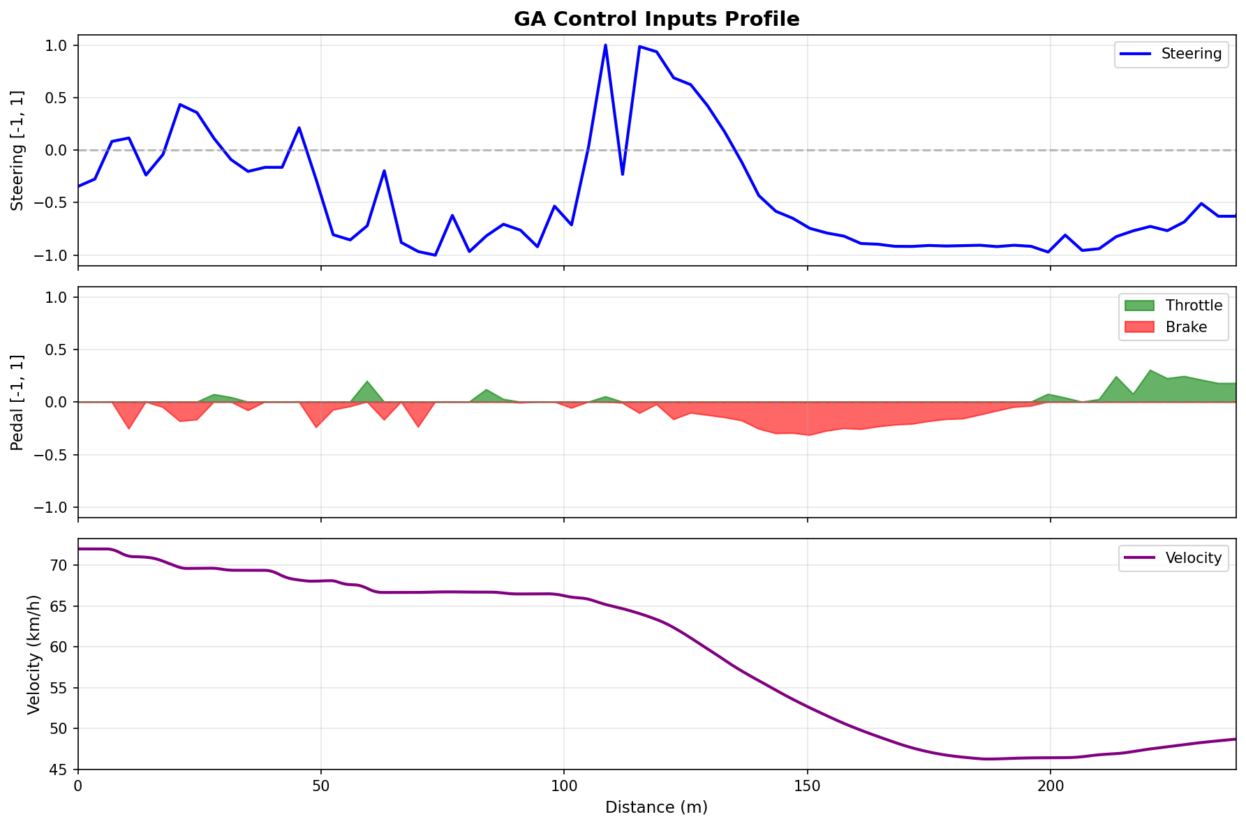
Step 5: Generating visualizations...
  ✓ Saved: results/ga_input_profile.png
  ⚠ Skipping G-G diagram (simulation didn't finish)
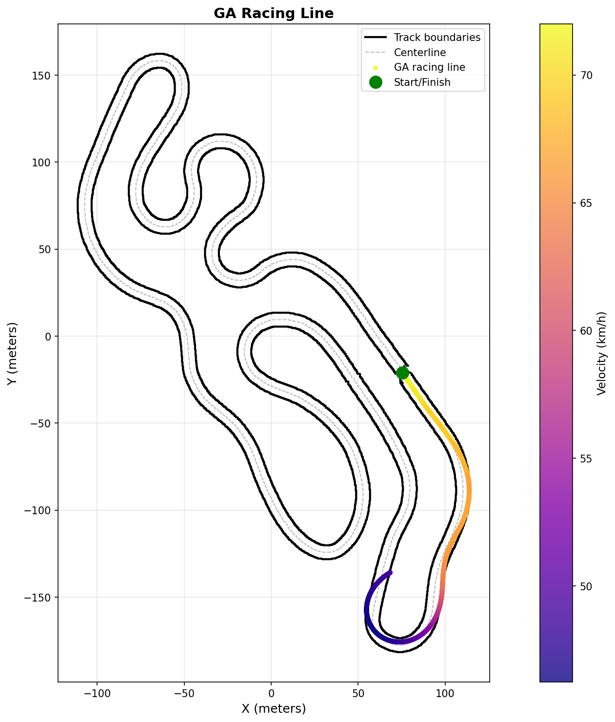
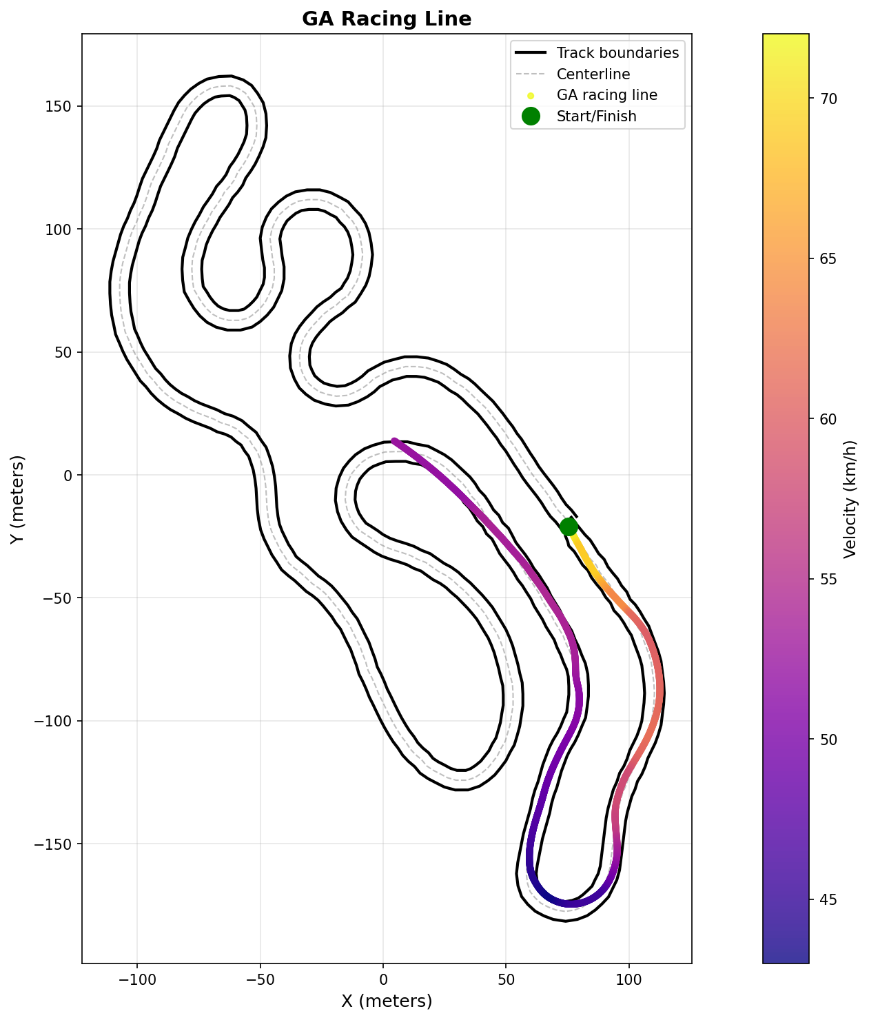
  ✓ Saved: results/ga_convergence.png
  ✓ Saved: results/ga_racing_line.png

Step 6: Exporting results...
  ✓ Saved: results/ga_best_chromosome.csv
  ⚠ Skipping detailed export (simulation didn't finish)
  ✓ Saved: results/ga_report.txt

============================================================
  EVOLUTION SUMMARY
============================================================
============================================================
  ApexSim GA-Edition - Evolution Report
============================================================

TRACK INFORMATION
  Length: 1781.88 m
  Points: 2651

VEHICLE PARAMETERS
  Top Speed: 85.0 km/h
  Max Lateral G: 1.0g
  Max Braking G: 0.6g
  Max Accel G: 0.3g

GA CONFIGURATION
  Population Size: 200
  Elitism: 10
  Crossover Prob: 70.0%
  Mutation Prob: 20.0%
  Control Nodes: 392

EVOLUTION RESULTS
  Generations: 100
  
  Initial Best Fitness: 1706.90 s
  Final Best Fitness:   1643.77 s
  
  Improvement: 63.13 s (3.7%)

BEST LAP DETAILS
  Finished: False
  Lap Time: 1643.76 s

============================================================

Total evolution time: 3.1 minutes
Time per generation: 1.8 seconds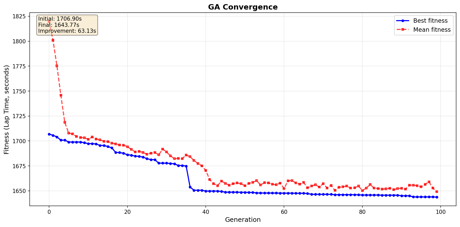

After some training, it learn this:

This was… promissing?

Something was off, why despite feeding the fastest route (actions) from the GD simulation done before am i getting crashing evolutions?

Discrete to Continuum

The genetic algorithm works with discrete control points, but the racing line needs to be converted to a continuous representation for the physics simulation.

This conversion is crucial for the GA to effectively optimize the racing line.

The conversion process involves interpolating between the discrete control points to create a smooth, continuous racing line that can be accurately simulated by the physics engine.

Lets be realistic…commanding a kart once every for meters wont got you far.

cd 1-pointmass-lap-gradient-based/
python3 visualize_track_splines.py #see track_spline_structure.png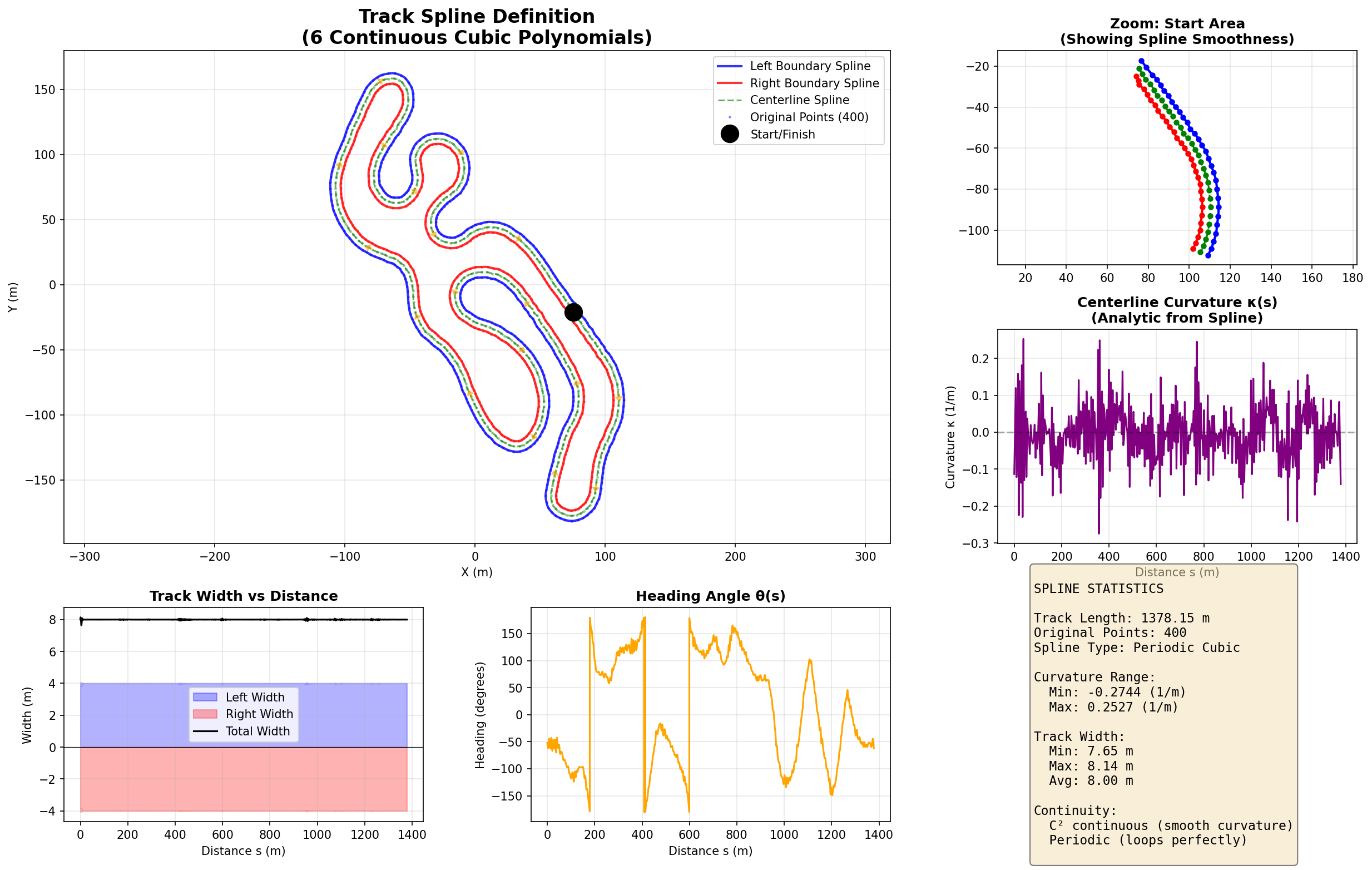

Here is when it comes that moment that brings you back to calculus or mechanincs lessons back in time.

There are no N curves in a circuit, there are infinite curves, each with their radious and center somwhere in the space.

Here is the top 20 of changes in curvature: which should normally be the entries/exits of what we tend to call turns of the circuit

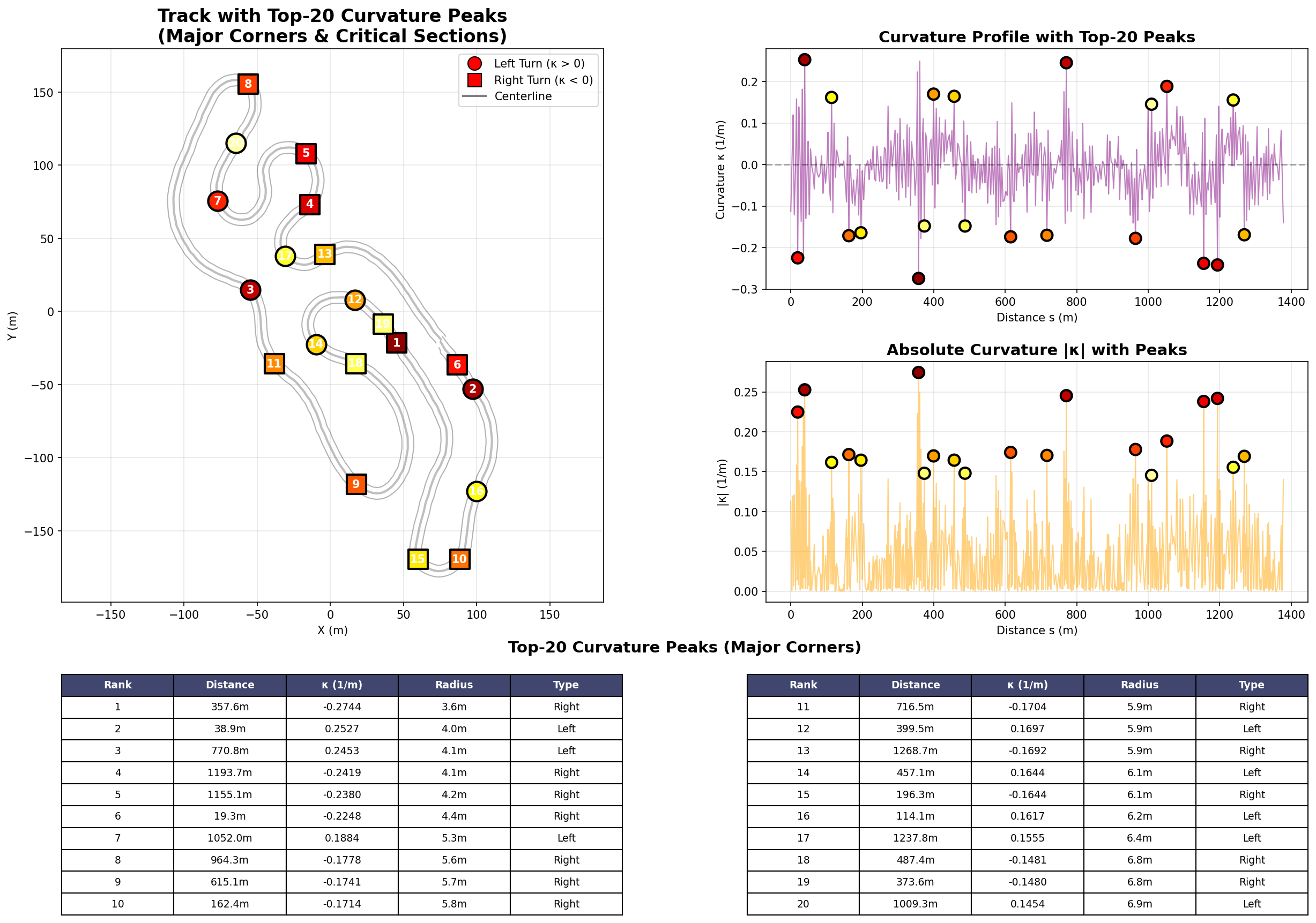
You might see some like top 6 and top 1 that represent nothing - they are there because of noise in the discrete data to make the continuum.

From this point, I wanted to test how good the continuum was.

MCP as better seed?

No, not the model context protocol!

This is…different.

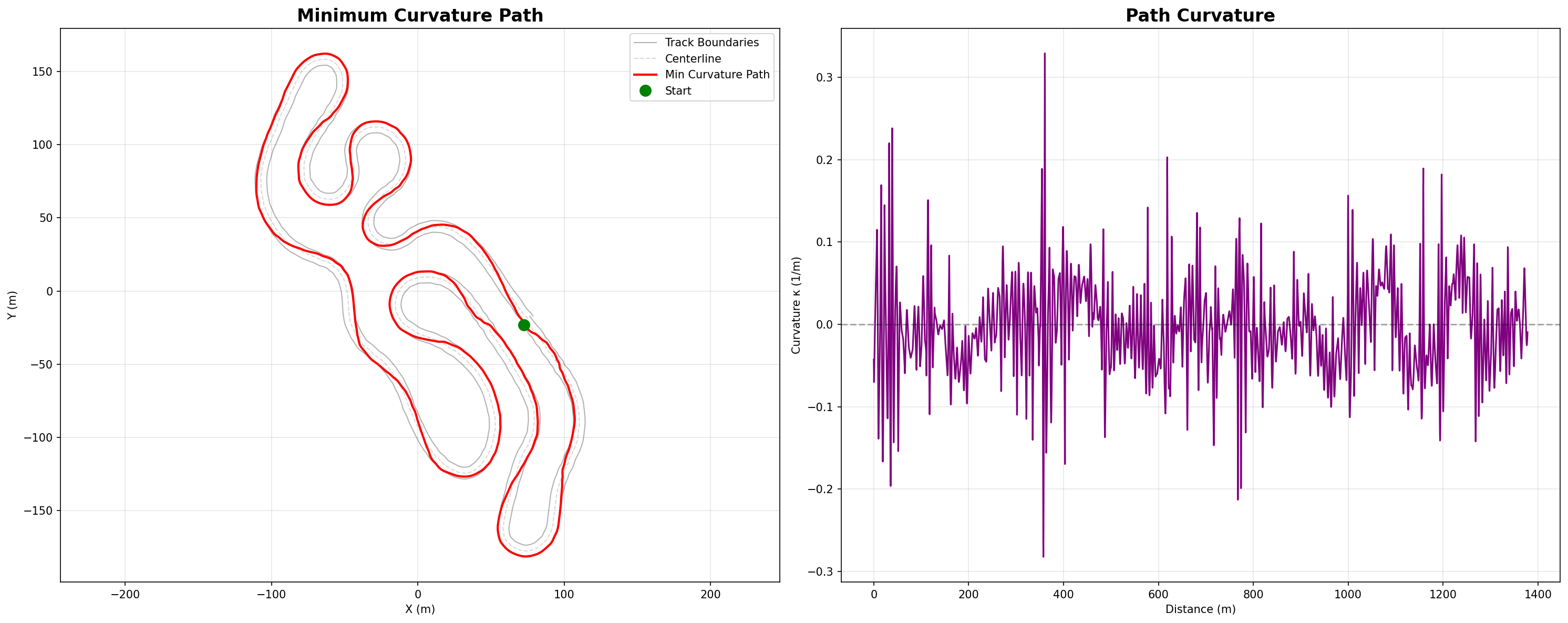
So just made a side quest to create the Minimum curvature path but with a continuum, not a discrete circuit

The idea here is to provide a better seed for the genetic algorithm chromosome.

#cd 0
python3 compute_min_curvature_path.py

This will run for a while and get you the path: optimized for a smoother low curvature, not for lap time

python3 compute_velocity_profile.py

This goes much faster as its just to apply the phyisical limits:

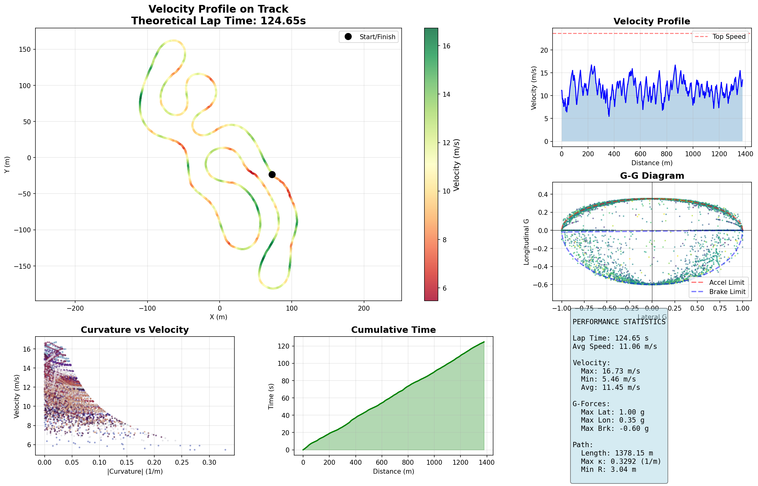
Theoretical best lap time: 124.65 seconds as per MCP, far worst than GD that went straight away for the ~80s validated IRL

• Average speed: 39.8 km/h

python3 export_actions.py #and we get a csv with the distance, speed, actions...

How could I not: using the previous csv outputs

python3 create_lap_animation.py
#python3 create_lap_animation_v2.py

Which goes to min_curvature_actions_5000.csv

I improved the UI on a v2 version of it.

python3 validate_with_simulation.py

And…it crashed at around 68m/1300m.

Interesting, but if that trajectory…was smooth (?)

So…given that the MCP path was smootha and i got the actions: how about creating the path that those actions create given the current physics engine?

python3 simulate_and_check_path.py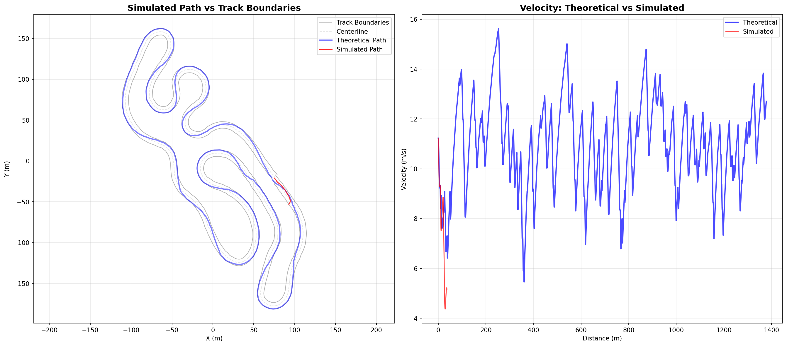

Conclusions

The physic engine simulator paid off.

This is a fundamental physics difference - it models power-limited acceleration (like a real engine) rather than force-limited acceleration.

I got inspired by:

and its code https://github.com/kleberandrade/evolve-kart-unity

FAQ

Taylor vs Splines?

Are theused splines polynomials? Like Taylor series?

Yes, but different!

• Cubic splines are piecewise polynomials (degree 3 between each pair of points)
  • Cubic splines use many small cubic polynomials connected smoothly
  • Splines stay accurate everywhere by using local polynomials
• Taylor series approximates a function around ONE point using infinite terms
  • Taylor series can diverge far from the expansion point

Cubic splines use many small cubic polynomials connected smoothly

Key difference:

Taylor: $f(x) = a_0 + a_1x + a_2x^2 + a_3x^3 + …$ (one polynomial, many terms)

Cubic Spline: Many cubic polynomials $p_i(s) = a_i + b_is + c_is^2 + d_is^3$ connected at “knots”

Why splines are better for tracks:

Heading angle vs Curvature

The heading angle represents the direction the vehicle is pointing, while curvature represents how sharply the path is bending. These are related but distinct concepts.

The relationship between them is given by the derivative of the heading angle with respect to arc length, which equals the curvature.

3. How do we define heading angle?

Line 149: heading = np.arctan2(dy_center, dx_center)

Where:

dx_center = track.spline_x(s, 1) = derivative $\frac{dx}{ds}$ dy_center = track.spline_y(s, 1) = derivative $\frac{dy}{ds}$

Mathematically:

$$\theta(s) = \arctan2\left(\frac{dy}{ds}, \frac{dx}{ds}\right)$$

This gives the tangent direction (which way the car is pointing) at any distance $s$.

4. Why is curvature measured in 1/meters?

curvature = (dx_center * ddy - dy_center * ddx) / (dx_center**2 + dy_center**2)**1.5

Curvature $\kappa$ measures “how much the path curves”:

$$\kappa = \frac{1}{R}$$

Where $R$ is the radius of curvature (radius of the circle that best fits the curve at that point).

Units:

If $R = 100$ meters (gentle curve), then $\kappa = 0.01$ (1/m) If $R = 10$ meters (sharp turn), then $\kappa = 0.1$ (1/m)

Why 1/m makes sense:

Straight line: $R = \infty$, so $\kappa = 0$ (1/m)

Tighter curve: smaller $R$, larger $\kappa$

The formula (Frenet-Serret):

$$\kappa = \frac{x’y’’ - y’x’’}{(x’^2 + y’^2)^{3/2}}$$