Just maps v2
TL;DR
Doing cool stuff with geo data, sun and blender
Intro
Coming from this post
Ive seen ppl doing cool stuff with: blenderGis adon, maplibre and maptiler and f4map
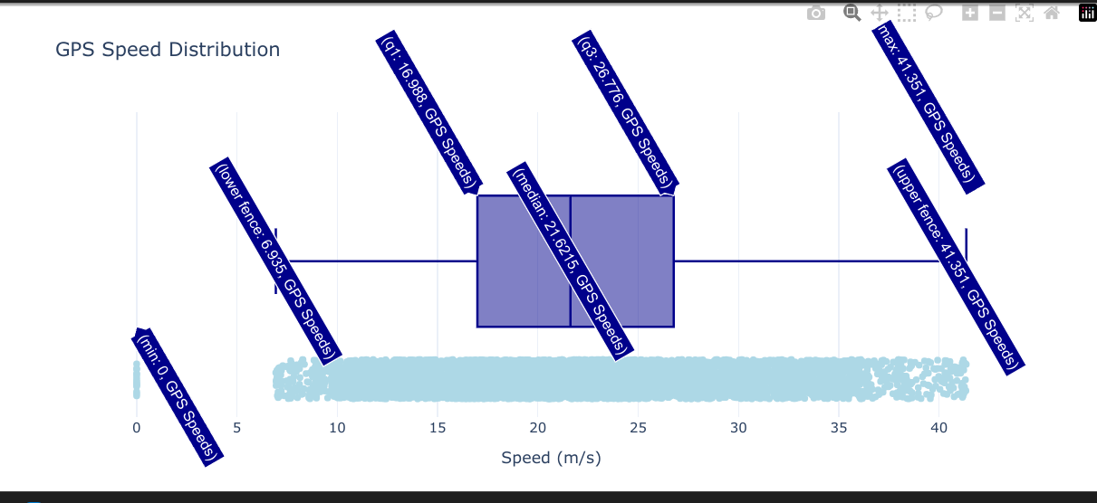 TrackDays and GoPro Telemetry
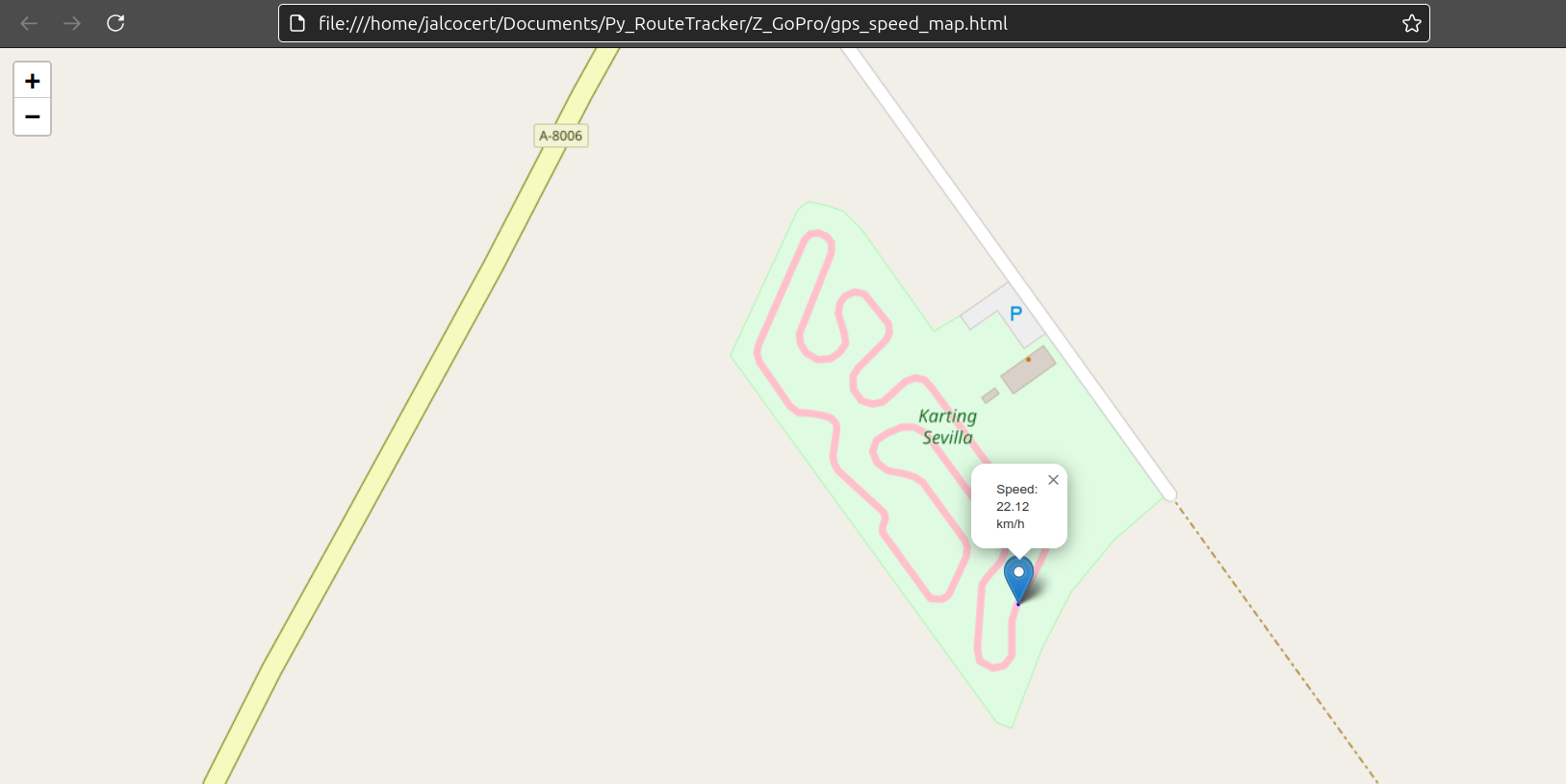 GoPro MetaData Magic 101
This is a good chance to:
- To have a look to French Real estate again:
Go to the details of DFV geo exploration
To check how household income is evolving in spain as a recap of this post
To use PyRouteTracker against more karting or trackday data:
candump turned off the car before going to spaJust imagine how a FPV Drone Telemetry x GPS could be!
Phyphox take off data: remember that you can configure replicable experiments via QR!
cd ./poc/airplane-phyphox- To think how the solar rays simulations of a building need more context of their surrounding:
#sudo snap install blender --classic --channel=5.1/stable
#cd ./poc/building-to-blender
#claude --dangerously-skip-permissions
cd ./poc/building-geo-to-blender| Date | Astronomical daylight | Direct sun | Lost to terrain |
|---|---|---|---|
| 21 Dec 2026 | 8.8 h | 3.3 h | 62% |
| 1 Jul 2026 | 15.0 h | 12.0 h | 20% |
Go to the details
- Matching an action cam video to a GPX file: the physics of coasting behind an ebike
SelfHosted GPX
- GPXStudio - https://github.com/gpxstudio/gpx.studio
MIT | the online GPX file editor
GeoLibre - https://github.com/opengeos/GeoLibre that you can find https://geolibre.app/
Dawarich - with Android app
You have several integrations http://localhost:3333/settings/integrations like with Velomate
Make sure to have proper Application hosts in the .env
on a fresh self-hosted install you should be able to sign in with the seeded default account:
- Username:
demo@dawarich.app - Password:
safepassword(github.com (https://github.com/Freika/dawarich))
For Cloudflare exposure, the important bit is that the app container must join the shared tunnel network, and Rails must allow the public hostname in APPLICATION_HOSTS.
- If you expose the same service both locally and through Cloudflare, the local port mapping can stay in place. The tunnel just adds another path in.
- The tunnel side does not need a separate reverse proxy here; your existing cloudflared container can route directly to dawarich_app:3000.
- Browser issues can look like app failures, but in this case the service was fine; the problem was the client path and DNS/IPv6 timing.
#network -> container name
docker network connect cloudflared_tunnel dawarich_app
#docker inspect gitea --format '{{json .NetworkSettings.Networks}}' | jq
Go to CF and add dawarich_app:3000
Geolibre
Owntracks
Others:
https://github.com/mendhak/gpslogger/
https://github.com/dietrichmax/colota
https://github.com/dawarich-app/atlas
Mobile GPX Apps
https://apps.apple.com/us/app/open-gpx-tracker/id984503772
- Dawarich
https://play.google.com/store/apps/details?id=com.zeitflow.dawarich&pli=1
GoPro GPS
https://box2overtake.com/blog/pitlane/#try-it https://github.com/jlleongarcia/Py_RouteTracker https://pitlane.box2overtake.com/
Building around GeoData
French DFV Prices x Geo
If you like housing analytics and you live in France, you are in paradise:
python scripts/build_transaction_map.py
start maps\dvf_eaux_bonnes_2025_transactions.html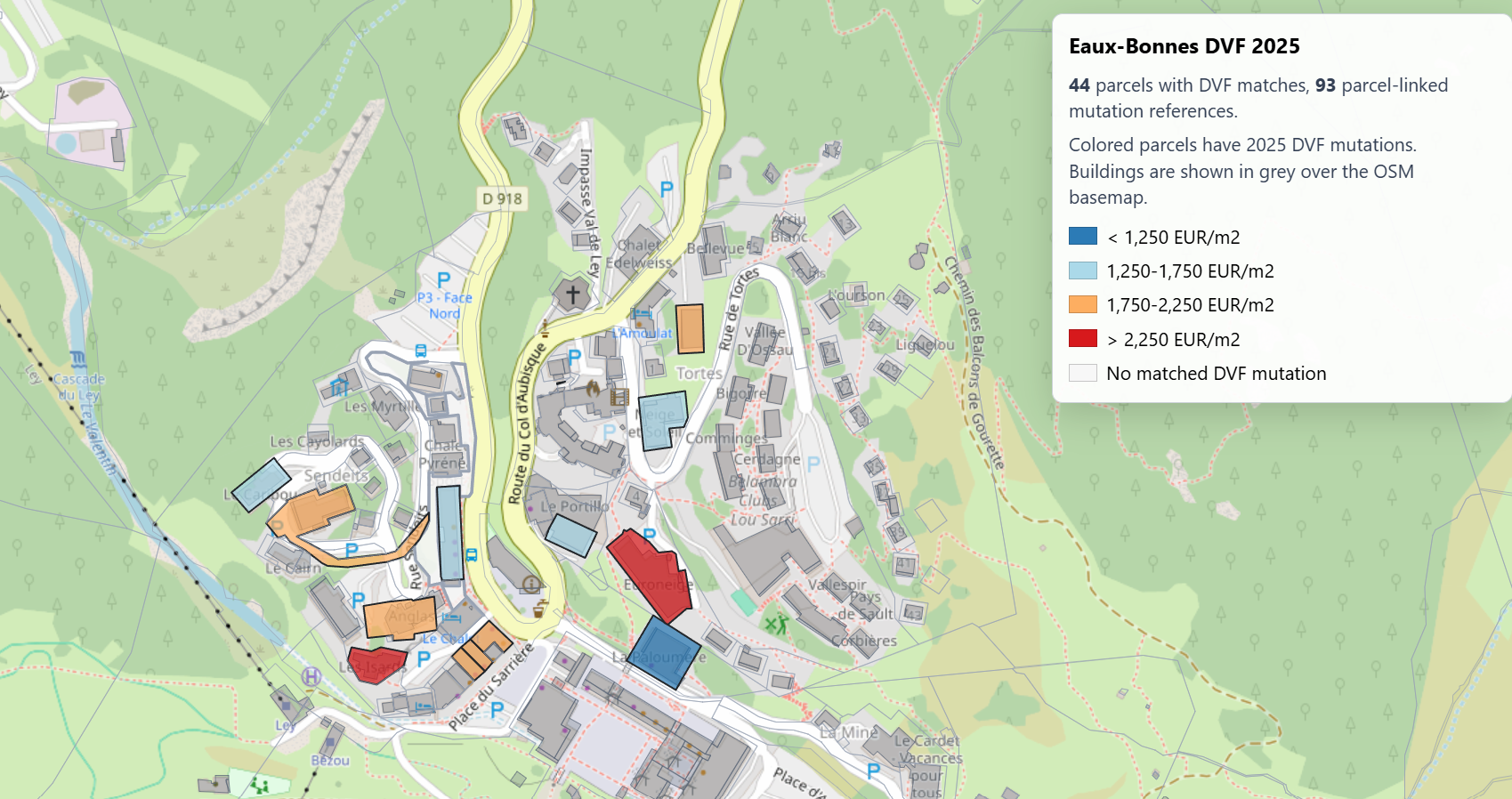
python scripts/build_france_transaction_map.py --max-mutations 1000
#  python scripts/build_france_transaction_map.py --department 64
maps\dvf_france_2025_transactions_preview.html

#start maps\dvf_france_2025_transactions_preview.html
start maps\dvf_combined_lyon_dept64_2025_transactions_preview.html
I put together a quick video here around those
python -m py_compile scripts\build_price_video.pySee where the sold houses are and how much sun they are getting in December, by combining: 22.8% of the inhabited corridor gets zero direct sun in December.
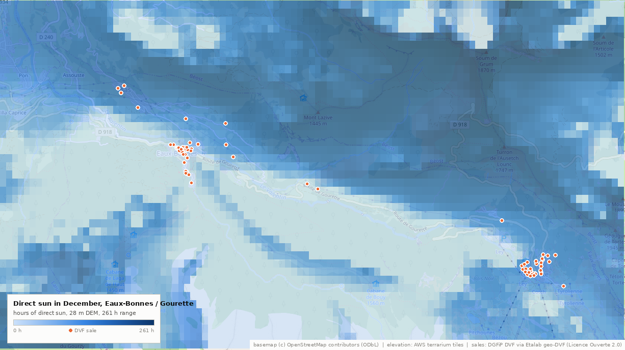
Roughly nine steps, and the ordering has one non-obvious dependency: the prices decide how big the DEM has to be, so you can’t fetch terrain first.
Pass 1 — the transaction study
1. Probe the source before writing anything. curl -sI on files.data.gouv.fr/geo-dvf/latest/csv/{year}/communes/64/64204.csv to find out what actually exists. Result: 2021–2025 only (latest is a rolling five-year window; 2014–2020 all 404). That single check decided the sample size for everything downstream.
2. Look at raw rows before designing the €/m² rule. Downloaded the five files (~180 KB total) and dumped a few multi-row mutations. That’s where the rule came from: Dépendance rows carry no surface_reelle_bati at all, so Appartement; Dépendance is one flat sold with its cellar — keep it, and use the flat’s surface as the denominator. Had I written the ingest first I’d have excluded those and thrown away most of the sample.
3. Ingest → fetch_geodvf.py. Group by id_mutation (the official key — no date+value+address heuristic needed), apply the pricing rule, log a reason for every rejection. → 485 mutations, 481 geocoded, 397 priced, median 1686 €/m².
4. Now size the terrain from the prices. Bbox of the transaction coordinates: 3.1 × 6.9 km, furthest point 3.8 km from centre. Since the horizon march needs 30 km, the DEM radius must be 30 + 3.8 ≈ 34 km. That’s the dependency — terrain extent is a function of where the sales are.
5. DEM fetch → fetch_terrain.py (copied verbatim from building-geo-to-blender). 110 terrarium tiles, 34 MB, 80 s, no API key, no GDAL.
6. Horizon per parcel → sun_by_point.py. The one piece of genuinely new geometry: the sibling project marches rays from the centre of its DEM, this marches from an arbitrary offset inside a shared one. Deduped to 117 distinct coordinates rather than 481 mutations, because DVF geocodes to the parcel. 17 s.
7. Join and test → join_analyze.py. Correlations, cluster-robust regressions, the faceted scatter, the Leaflet map. → the null result, which I then blamed on a +0.92 elevation/sun collinearity.
geo-DVF csv ──> mutations.csv ──┬──> bbox ──> DEM ──> horizons ──> sun_by_point.csv
                                │                                        │
                                └────────────────  join  ────────────────┘
                                                     ↓
                                        findings.json, chart, map
Pass 2 — the raster that overturned step 7’s diagnosis
8. Same DEM, grid instead of points → build_sun_raster.py. 4 515 cells, 5 min 20 s. Then — before trusting a single number — cross-check: sample the raster at the 117 parcel coordinates and compare against pass 1. r = 0.999, mean absolute difference 1.5 h, signed difference −0.05 h.
9. Bin by elevation → analyze_bands.py. This is where the reframing happened: over the terrain the collinearity is only +0.24, versus +0.74 over sold parcels and +0.92 over sales. So the matched-elevation test became possible, and it made the null stronger.
10. Composite → composite_map.py. Blend the raster onto real OSM tiles. Nominally an illustration; actually the georeferencing check — the pale corridor lands exactly on the Valentin and the D918.
The shape underneath it
Three habits did most of the work, and they’re all lifted from your existing projects rather than invented:
Inspect the data before writing the parser. Steps 1 and 2 each changed the design.
Two independent paths, then check they agree. Your
building-geo-to-blendercross-checks its analytic horizon against a Cycles render (38.4% vs 38.9%); here the raster cross-checks the point run, and the composite cross-checks the georeferencing. Every expensive claim has a cheap second opinion.Refuse rather than degrade. Both the point script and the raster script exit with the march radius that would fit instead of letting rays edge-clamp — because edge-clamping silently flattens distant ridges into a sunnier answer and leaves no trace in the output.
Stack: Python stdlib for the data plumbing, numpy for the marching, scipy for the statistics, Pillow for the rasters, matplotlib for the charts, Leaflet for the maps. No database, no GDAL, no npm.
Solar Rays x Buildings in a Geolocation
For an off-grid or heat-pump build, annual totals are the wrong statistic and December is the whole design constraint.
Yep, the sun is interesting.
Blender x GIS
And with blenderGIS you can create interesting simulations:
cd ./poc/blender-Video x GPX matching
Coasting behind an ebike
The amount of power (assistance) an e-bike provides depends on the motor rating, the jurisdiction/legal limits, and the difference between continuous vs. peak power.
- Typical Power Ratings (Nominal / Continuous)
- 250 Watts (Standard / EU, UK, Australia): In Europe, the UK, and Australia, the legal maximum for a standard pedal-assist bike (pedelec) is 250 W continuous rated power.
- 500 W to 750 Watts (US & Canada): In the United States and Canada, legal e-bikes (Class 1, 2, and 3) typically allow up to 750 W of nominal motor power.
- 1,000 W+ (Off-Road / Speed Pedelecs / DIY): High-power cargo bikes, speed pedelecs, or off-road e-bikes range from 1,000 W up to 1,500 W+.
- Nominal (Continuous) vs. Peak Power
Advertised motor wattage usually falls into two categories:
| Type | What It Means | Typical 250W Bike | Typical 750W Bike |
|---|---|---|---|
| Nominal (Continuous) Power | The power the motor can output continuously without overheating. (Used for legal compliance). | 250 W | 750 W |
| Peak Power | Short bursts of max power during heavy acceleration or steep hill climbing. | 400 W – 600 W | 1,000 W – 1,300 W |
- Human Power vs. E-Bike Power
To put e-bike assistance in perspective relative to human effort:
- Average Human Cyclist: Produces around 100 W to 150 W of sustained pedaling power.
- Fit / Amateur Cyclist: Produces around 200 W to 250 W.
- Pro Cyclist: Sustains 350 W to 450 W during intense efforts.
You can imagine how hard was to cross from UK to FR by a bike powered plane!
For a non-professional cyclist, power output depends heavily on fitness level, body weight, and duration.
Cycling power is typically measured at FTP (Functional Threshold Power—the maximum average wattage you can hold for roughly 1 hour)
or measured in Watts per kilogram ($\text{W/kg}$).
Sustained Power (1-Hour Continuous Effort)
For an average adult male weighing around $75\text{ kg } (165\text{ lbs})$:
| Fitness Level | Sustained Power (FTP) | Relative Power ($\text{W/kg}$) | What That Looks Like in Real Life |
|---|---|---|---|
| Untrained / Casual | $100\text{ – }150\text{ W}$ | $1.3 \text{–} 2.0\text{ W/kg}$ | Commuting, casual gym bike, easy recreational riding. |
| Recreational | $150\text{ – }200\text{ W}$ | $2.0 \text{–} 2.7\text{ W/kg}$ | Rides 1–2 times a week, can maintain $20\text{–}24\text{ km/h}$ on flat road. |
| Fit Amateur (Club Rider) | $200\text{ – }260\text{ W}$ | $2.7 \text{–} 3.5\text{ W/kg}$ | Trains regularly, does weekend group rides, fast on flats. |
| Strong Amateur Racer | $260\text{ – }320\text{ W}$ | $3.5 \text{–} 4.2\text{ W/kg}$ | Competes in local races (Cat 3/4), very fast on climbs. |
Short-Burst / Sprint Power
If you ask a non-professional to stomp on the pedals as hard as possible for a brief burst:
- 5–10 Second Max Sprint: An average non-pro can burst $500\text{ to }900\text{ Watts}$. A strong amateur sprinter can peak around $1,000\text{ to }1,200\text{ Watts}$.
- 1-Minute Hard Effort: A healthy non-pro can hold $300\text{ to }450\text{ Watts}$ before severe fatigue and acid buildup set in.
Bike Reverse Engineering Experiment
I remember that we made an experiment during the studies where we logged bike sensor data
- https://github.com/JAlcocerT/hermesagent/tree/tinker/hermesagent/mbsd/bike-practicas-cdm
- https://github.com/JAlcocerT/mbsd/tree/master/bike-practicas-cdm-python
This can be useful to estimate the power i applied to the bike
git clone JAlcocert/hermesagent/
cd ./tinker/hermesagent/mbsd/bike-practicas-cdm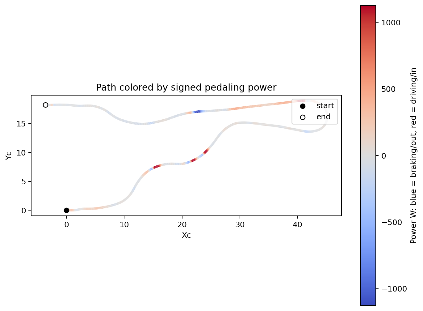
Conclusions
Not sure about you, but im doing:
flowchart LR
    %% --- Styles ---
    classDef free fill:#E8F5E9,stroke:#2E7D32,stroke-width:2px,color:#1B5E20;
    classDef low fill:#FFF9C4,stroke:#FBC02D,stroke-width:2px,color:#FBC02D;
    classDef mid fill:#FFE0B2,stroke:#F57C00,stroke-width:2px,color:#F57C00;
    classDef high fill:#FFCDD2,stroke:#C62828,stroke-width:2px,color:#C62828;
    classDef bridge fill:#E3F2FD,stroke:#1565C0,stroke-width:3px,color:#0D47A1;

    %% --- Nodes ---
    L0("Free Content
( DIY = $0)"):::free
    L1("Web Audits 🛡️
(Reveals Problem )"):::free
    L11("Tech Blog/Youtube"):::free
    L12("ebooks"):::free
    L13("mbsd framework OSS"):::free
    L14("OSS guides"):::free

    L3("Done With You
(Trade $$ for knowledge)"):::mid
    L4("Done For You
(Trade $$$ for outcomes)"):::high
    L44("GenBI
Shopify PoC"):::bridge
    L45("Real Estate
Funnel Bot"):::bridge
    L46("Energy Solutions
HVAC"):::bridge
    L47("IoT Solutions
Crops"):::bridge
    L48("Weddings
Photo QR"):::bridge

    %% --- Connections ---
    L0 --> L1
    L1 --> L3
    L12 --> L3
    L13 -->|MultiBodySystemsDynamicscom| L3
    L14 -->|FOSS Engineer| L3
    L0 --> L11
    L0 --> L12
    L0 --> L13
    L0 --> L14
    L3 --> L4
    L4 -->|Productized Service| L44
    L4 -->|Productized Service| L45
    L4 -->|Productized Service| L46
    L4 -->|Productized Service| L47
    L4 -->|Productized Service| L48
FAQ
Finding interesting housing data
- For Spain
You can correlate with household income
For FR:
For DK:
For PL: