Optimum Path in Karting x ApexSim
TL;DR
A simple starting model to find the optimum path while racing.
Intro
Based on the gopros data and videos you can find online, you can see whats the G-circle model is all about.
See that generally a kart can accelerate up to: ~0.3G
Brake up to: ~0.5g and turn up to: ~1G
    "vehicle": {
        "top_speed_kmh": 85.0,
        "initial_speed_kmh": 72.0,
        "max_lateral_g": 1.0,
        "max_braking_g": 0.6,
        "max_accel_g": 0.35,
        "mass_kg": 230}
Sodikart RX250 typically weighs approximately 135 kg to 150 kg
No need to get a mycron 5s so far, just lets do some simulations to understand the potential flying laps.
 Tinkering with Racing and GoPro GPS
 NEW - Optimum Path Repo
We come from some previous tinkering on racing:
With interesting results:
Arriving here?
Just after a few posts on action cams and GPS data within this repo.
Optimum path in karting
This is a great moment to step back and look at the “Architecture” of a karting simulator.
Moving from raw data to a high-level optimization problem.
In real life unlike (apparently) in modern economics if you assume that a spherical cow will fly - you will be laughed at (and fail quickly).
This is going to be simple, let’s optimize for: the minimum possible lap time!
$$\int ds/v(s)$$
While keeping our braking, accelerating $a_accel(v) = a_0 · (1 - v/v_max)$ and cornering limits realistic.
So these strategies to estimate that fastest lap have all HYPOTHESIS with pros/cons.
- The Data Foundation (The Input)
- Source: CSV file containing track limits. From the Go Pro GPS
- Hypothesis: The physical limits of the kart are constant, but acceleration decreases as a function of speed: a=f(s)
- Pros: CSV is universal and easy to manipulate in Python.
- The Physics Models (The “Engine”)
We discussed two ways to treat the kart:
| Model | Hypothesis | Pros | Cons |
|---|---|---|---|
| Point Mass (G-G Circle) | The kart is a single dot. Grip is a perfect circle (or ellipse). | Very fast to calculate; requires very little data. | Ignores weight transfer, chassis flex, and tire “scrub.” |
| Bicycle Model | Accounts for CG height and weight transfer. | More realistic “yaw” (rotation) modeling. | Requires more measurements (CG height, wheelbase). |
- The Path Strategies (The “Line”)
This is where the actual “lap time” is found.
Option A: Minimum Curvature Path (MCP)
- Hypothesis: The fastest way is the “smoothest” way (maximizing radius), hence with higher speed throughout the corner and better grip utilization.
- Pros: Mathematically elegant; very fast to solve; much better than a centerline.
- Cons: Ignores the “Late Apex” advantage. It treats a 10m straight and a 100m straight the same way, which is not true!
Option B: Late Apex (Momentum/Time Bias)
- Hypothesis: Sacrificing mid-corner speed for a straighter exit wins time on long straights.
- Pros: This is how professional drivers actually drive.
- Cons: Harder to calculate with a simple formula; requires “looking ahead” at the track.
- The Solver (The “Brain”)
The good news is that we have the power to choose how to find the best line:
The Genetic Algorithm (GA) — Recommended
How it works: Evolution. It tries 100 lines, keeps the 10 fastest, “mutates” them, and repeats.
Pros: * It will “discover” the late apex on its own because it only cares about the lowest time.
Easy to code in Python (
PyGADorNumPy).Perfect for your 5600G (you can run 12 “generations” at once).
Cons: Can take a few minutes to converge on the “perfect” lap.
Neural Networks / Reinforcement Learning
- How it works: An AI “agent” drives the kart millions of times to learn the limits.
- Pros: Can handle very complex physics (sliding, grass, etc.).
- Cons: Massive overkill for a point-mass model; very high “coding cost” to setup the environment.
Summary to recap:
- Format: everything to CSV.
- Physics: Use the G-G Ellipse (allowing more braking Gs than acceleration Gs) combined with an acceleration decay function.
- Pathing: Use a Genetic Algorithm.
- Use Splines (don’t optimize every point, just “control points”).
- Use Vectorization (NumPy) so a ~ 5600G CPU can calculate 1,000 laps per second.
- The Result: This will give you a “Theoretical Best” lap time that accounts for the specific top speed (85 km/h) and power drop-off of your kart.
The mass point model + Gradient based optimization
A mass and a gradient based optimization…
to get started: Optimum Path 101
#sudo apt install gh
gh auth login
#gh repo create make-podcast --private --source=. --remote=origin --push

git init && git add . && git commit -m "Initial commit: simple optimum path" && gh repo create optimum-path --private --source=. --remote=origin --push
Minimum Curvature Path (MCP): not the AI MCP, but the curvature one
- Optimizes: Smoothness
- Fast but wrong objective for racing
- Good for initialization only
Gradient-Based Optimization (ApexSim):
- Optimizes: Lap time
- Slow but correct objective for racing
- What you actually care about!
ApexSim uses gradient-based optimization because: The ApexSim’s Design Choice
- ✅ We want to minimize lap time, not curvature
- ✅ We have vehicle physics data (G-limits, power, mass)
- ✅ Computation time (minutes) is acceptable for analysis
- ✅ We need realistic racing lines that consider physics
- ✅ Cubic splines are used for smoothing, not optimization
- MCP: Minimizes
∫ κ² ds(curvature) using gradient descent - ApexSim: Minimizes
∫ ds/v(s)(lap time) using SLSQP
#python3.10 1-pointmass-lap-gradient-based/apexsim_v1.py
cd 1-pointmass-lap-gradient-based/
python3.10 apexsim_v1.py #configured as per vehicle_config.json including the track
$$\int ds/v(s)$$
Conclusions
Im impressed on how a simple model can provide realistic results.
A point with all the mass of the kart and the driver.
Some Newton and G-circle…and the gradient descent does the trick.
The results
After few iterations to get the components rendered in a nicer way:
A simple mass + no multi body, no contact dynamics with those slip angles, no aerodinamics, no ICE modelling with its volumetric efficiencies, no kart flexing…
Just…a point with a good enough model and parameters that can be validated from the real go pro videos on board.
"vehicle": {
    "top_speed_kmh": 85.0,
    "initial_speed_kmh": 72.0,
    "max_lateral_g": 1.0,
    "max_braking_g": 0.6,
    "max_accel_g": 0.35,
    "mass_kg": 230,
    "comment": "Typical rental kart parameters. Adjust based on actual vehicle specs. Initial speed = entry speed for flying lap."
},
Plot twist 🤯: whatever happens in the circuit in real life prevails to ANY model results
Its all on this repo: https://github.com/JAlcocerT/optimum-path
Unfortunately, you wont have access, but can get some of my time if you want to learn how to create:

What else?
Since you have already built ApexSim using a gradient-based path optimizer, you have surpassed 90% of amateur simulation projects.
To go further, you must move away from “Steady State” (where we assume the kart is always balanced) and move toward Transient Dynamics (how the kart behaves while changing direction).
1. The “Optimal Control” Approach (The Mathematical “Holy Grail”)
Instead of optimizing a path and then calculating speed, you treat the entire lap as a single mathematical problem where you solve for Steering, Throttle, and Brake inputs simultaneously.
- How it works: You use a library like
CasADiorPyomoto solve a Nonlinear Programming (NLP) problem. Instead of “where should the kart go?”, the question is “what should the pedals and wheel do at every millisecond?” - Why it’s better: It naturally discovers “Slip Angles.” It might find that the fastest way through a corner is to enter with the rear slightly sliding (oversteer) to point the kart earlier—something your current model cannot do.
- The Physics: It uses a Bicycle Model with tire formulas (like the Pacejka “Magic Formula”) instead of a simple G-Circle.
2. Reinforcement Learning (The “AI Driver”)
Instead of solving equations, you let an AI “learn” to drive your kart through trial and error in a simulated environment.
- The Setup: Use
Gymnasium(OpenAI Gym) to create a track environment. The “Agent” (the driver) gets a reward for higher speed and lower lap time. - Why it’s better: An RL agent will find “creative” lines that a mathematical optimizer might miss, such as using specific curbs to rotate the kart or finding “hooks” in the track geometry.
- CPU Impact: Your AMD 5600G is perfect for this if you use “Stable Baselines3.” You can run multiple “environments” in parallel on your 12 threads to train the agent faster.
3. Thermal and Energy Management Simulation
In karting, your “best lap” isn’t just about geometry; it’s about Heat.
- Tire Temp Model: Tires provide maximum grip only within a specific temperature window. You can simulate the heat generated by friction () and how it degrades the over a 10-lap stint.
- Engine Heat/Fade: As the engine gets hotter, the function shifts downward.
- Why do this? This helps you simulate not just the single fastest lap, but the Fastest Race Strategy. It might tell you that being 0.1s slower on Lap 1 saves the tires enough to be 0.5s faster on Lap 10.
4. Comparison of Methods
| Method | Complexity | Best For… |
|---|---|---|
| Current (ApexSim) | Medium | Finding the “Ideal” line and theoretical limit. |
| Optimal Control | High | Modeling tire slip, drifting, and transient weight transfer. |
| Reinforcement Learning | Very High | Discovering non-obvious lines and “driving styles.” |
| Thermal/Multi-Lap | Medium | Race strategy and tire pressure management. |
If you want to stick to the “engineering” side, Optimal Control with a Bicycle Model is the logical next step.
It will allow you to see how the kart’s wheelbase and CG height actually affect the lap time.
If you want to see the “AI” in action, Reinforcement Learning is a fascinating rabbit hole that uses your hardware very effectively.
GA vs RL
Yes, they are fundamentally different “philosophies” of optimization. Think of it this way:
- Genetic Algorithm (GA) is about breeding the best path. * Reinforcement Learning (RL) is about training a driver.
Here is a breakdown of how they compare when applied to your Point-Mass model.
- The Genetic Algorithm (The “Evolutionary” Approach)
In your ApexSim context, a GA looks at the track as a whole. It treats the entire racing line as a “DNA strand.”
- How it works: It creates 100 random lines. It doesn’t “drive” them; it just calculates the lap time for all of them. It picks the fastest ones, mixes their “DNA” (segments of the path), and adds random mutations (nudging a point left or right).
- Knowledge: The GA has zero memory. If you change one corner, it has to evolve all over again. It doesn’t “understand” racing; it just understands that “Path A was faster than Path B.”
- End Result: You get a static file of coordinates that represents the perfect line.
- Reinforcement Learning (The “Neural” Approach)
RL doesn’t care about the “line” initially. It cares about the Policy—a set of rules in a Neural Network that tells the driver what to do based on what it sees.
- How it works: The “Agent” starts at the finish line and is told “Go.” It crashes 5,000 times. Each time it stays on track longer or goes faster, it gets a “Reward” (numerical points). The Neural Network adjusts its weights to maximize those points.
- Knowledge: The RL agent develops “Intuition.” It learns that “If the curvature is high, I must brake.” If you move the agent to a different track, it will likely drive it reasonably well immediately because it learned the principles of driving, not just one specific path.
- End Result: You get a trained model (a .zip or .pkl file) that can drive the kart in real-time.
- Comparison for your Point-Mass Kart
If your goal is purely to estimate the fastest lap time for your specific track:
| Feature | Genetic Algorithm (GA) | Reinforcement Learning (RL) |
|---|---|---|
| Setup Time | Easy. Just need your CSV and the fitness function. | Hard. Need to build a “Gym Environment.” |
| Compute Power | Efficient on your 5600G (Parallel math). | High. Needs thousands of episodes to “converge.” |
| Optimal Value | Very high. Usually finds the “Global Optimum.” | Can be “noisy.” Might settle for 99% of the limit. |
| Transferability | None. Only works for that specific track. | High. Can drive other tracks or handle rain/oil. |
- Which is better for you?
Since you already have ApexSim working with a Gradient-Based solver (which is mathematically closer to a GA), switching to RL would be a “lateral move” in terms of lap time accuracy, but a “vertical move” in terms of complexity.
- Stay with GA/Gradient: If you want the most accurate number for your track as quickly as possible.
- Move to RL: If you want to build an “AI Driver” that can react to other karts, changing grip levels, or if you want to eventually put this AI into a game or a real-time coach.
Yes, exactly. But the way they learn and use those percentages is the key difference.
To make this work for either a Genetic Algorithm (GA) or Reinforcement Learning (RL), you have to define the Action Space. Instead of just moving points, you are now controlling the “pedals” and the “wheel.”
For those 2 the model will have to learn on the % of braking % accelerating and % steering?
- For the Genetic Algorithm (GA)
In a GA, the “DNA” is a time-series of inputs.
The Chromosome: Imagine a giant spreadsheet where every 0.1 seconds you have a row for:
Steering %(-100% to +100%)Pedal %(-100% braking to +100% acceleration)The Process: The GA generates a random sequence of these inputs. The “Physics Engine” (your point mass model) executes them to see where the kart ends up.
The Problem: Most random sequences will just result in the kart driving straight into a wall or spinning in circles. The GA has to “evolve” the perfect sequence of steering and pedal inputs to stay on track.
- For Reinforcement Learning (RL)
In RL, the model doesn’t learn a “sequence.” It learns a Policy ().
The Input (Observation): At every moment, the AI looks at: “I am at 60km/h, the next corner is a right-hander 20 meters away, and I am 1 meter from the left edge.”
The Output (Action): The Neural Network calculates the best % for:
SteeringAcceleration/BrakingThe Learning: If the AI chooses 100% acceleration and 0% steering and hits a wall, the weights in the Neural Network are adjusted so it is less likely to do that again in that specific situation.
- Constraints: The G-G Circle Check
For both models, you must enforce your physical limits.
If the AI/GA tries to do 100% Braking AND 100% Steering at the same time, your code must intervene:
Calculate the Resultant Force: Use the Pythagorean theorem on the inputs.
Clip the Action: If , you must “clip” or scale the inputs down so they fit inside your G-Circle.
The Penalty: In RL, if the AI tries to exceed the G-limit, you give it a small negative reward to teach it that “scrubbing” the tires is inefficient.
Which is harder to learn?
- Steering is actually the hardest part for an AI to learn because a tiny mistake at the start of a corner leads to a massive crash at the end.
- Braking/Acceleration is easier because it’s a direct relationship with the function you already built.
Comparison of Control
| Feature | GA Control | RL Control |
|---|---|---|
| Input Type | A “Tape” of commands (Open Loop). | A “Brain” reacting to sensors (Closed Loop). |
| Stability | One bad “gene” ruins the whole lap. | Can recover from a slide or a mistake. |
| Precision | Great for finding the 100% theoretical limit. | Great for finding a “safe” and fast limit. |
For your specific goal—estimating the fastest lap time on a single track using a point mass model—the Genetic Algorithm (GA) makes much more sense.
While Reinforcement Learning (RL) is more “exciting,” it is often overkill for lap time estimation.
Here is the final verdict based on your project needs and your hardware (AMD 5600G).
- The Decision: Genetic Algorithm (GA) wins for Estimation
The GA is essentially a global search tool. Since you are looking for one specific answer (the absolute fastest line and set of inputs for one track), the GA is more efficient.
| Feature | Why GA is better for YOU | Why RL is likely unnecessary |
|---|---|---|
| Goal | You want the Global Optimum (the #1 fastest time). | RL often settles for a “good enough” policy that is 95% fast but safe. |
| Logic | GA breeds the best Line. Once it’s found, you’re done. | RL builds a Driver. You don’t need a driver; you need a result. |
| Speed | 100% of your 5600G power goes into finding the line. | Much power is “wasted” on the AI learning how to not hit walls. |
| Data | Works perfectly with your static CSV/NSP track limits. | Needs a “live” interactive environment to learn. |
- When would RL make more sense?
You should only switch to RL if your project goals change to:
- “I want an AI that can race against other karts.” (GA can’t handle dynamic opponents easily).
- “I want to see how a driver reacts to a tire puncture or rain mid-lap.”
- “I want to export a ‘brain’ into a game like Assetto Corsa or a real-time coach.”
- How to implement the GA “Action Space”
If you choose the GA, your “chromosome” (the DNA) shouldn’t be the coordinates anymore.
It should be the Control Inputs.
This makes the result “real.”
From the current 1st optimum path version generated with the GD version, we can have an idea of the actions that are been applied:
These are generated from the python3.10 apexsim_v1.py execution.
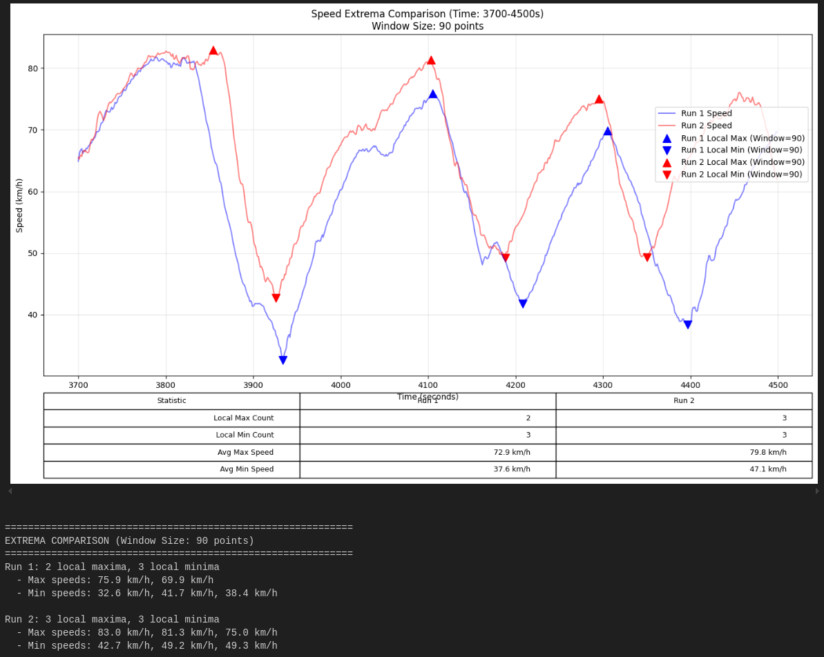
And how those reflect in the trajectory and speed distribution over time
Your DNA Structure:
An array of “Control Nodes” every 5–10 meters of the track. Each node has two genes:
- Steer Gene: Value from -1.0 to 1.0.
- Pedal Gene: Value from -1.0 (Full Brake) to 1.0 (Full Gas).
The “Physics Police” (The Ellipse Constraint): As the GA simulates the lap, it must check every step:
def physics_step(steer, pedal):
    # Calculate proposed Gs
    lat_g = steer * max_lat_g
    long_g = pedal * (max_brk_g if pedal < 0 else max_accel_g)

    # The Ellipse Check
    if (lat_g/max_lat_g)**2 + (long_g/max_long_g)**2 > 1:
        # Scale back to the edge of the ellipse
# This represents the tire "scrubbing" or reaching its limit- Final Verdict for ApexSim
Since you’ve already built a Gradient-Based optimizer, you are actually closer to a GA philosophy than an RL one.
My advice: Stick with your current Gradient-Based/GA approach. Refine your “Fitness Function” to use the Ellipse Constraint and the speed profile function. This will give you a mathematically perfect “Target Lap Time” that you can use to benchmark your real-world driving.
Would you like the Python code for the “Ellipse Clipping” function to ensure your GA/Optimizer never “cheats” the physics?
FAQ
Pacejka Magic Formula
The Pacejka Magic Formula is the gold standard in vehicle dynamics for modeling how tires generate force.
It was developed by Hans Pacejka and is essentially a semi-empirical mathematical formula that describes the relationship between tire deformation (slip) and the resulting force.
In your ApexSim model, you currently treat grip as a “binary” limit (you either have it or you don’t). In the Pacejka model, grip is a curve.
- The Core Concept: Slip
Tires do not work like rigid blocks. To generate force, the rubber must “slip” or “creep” against the road.
- Slip Angle (): The difference between the direction the wheel is pointing and the direction the kart is actually moving. This generates Lateral Force ().
- Slip Ratio (): The difference between the rotational speed of the tire and the actual forward speed (e.g., during burnouts or heavy braking). This generates Longitudinal Force ().
- The “Magic Formula” Equation
The formula is called “Magic” because it can fit almost any tire data using a set of coefficients (). The general form for the force () as a function of slip () is:
Each coefficient controls a specific physical characteristic of the tire:
| Coefficient | Name | Physical Meaning |
|---|---|---|
| D | Peak Value | The absolute maximum grip (the “ceiling” of the curve). |
| C | Shape Factor | Determines the “stiffness” and how aggressively the curve drops after the peak. |
| B | Stiffness Factor | How quickly the tire gains grip as you start to turn the wheel. |
| E | Curvature Factor | Controls the shape around the peak (how “forgiving” the tire is at the limit). |
- Why this matters for your Kart
In a kart, the Pacejka model reveals several behaviors your current Point-Mass model misses:
- The “Limit”: In ApexSim, if you exceed , the simulation simply says it’s impossible. In Pacejka, if you exceed the optimal slip angle (usually to ), the grip drops off. This is why karts “slide” and lose time if you turn the wheel too much.
- Self-Aligning Torque: The model also calculates the force trying to straighten the steering wheel. This is crucial if you ever want to simulate the physical effort required by the driver.
- Load Sensitivity: Pacejka models show that as you put more weight on a tire, it gains grip, but at a diminishing rate. This is why karts use “jacking” (lifting a wheel) to manage the differential effect.
- Integration into ApexSim
To use this in a simulation, you would replace your constant with a lookup or a function call:
- Calculate current Slip Angle based on velocity and steering input.
- Input that angle into the Pacejka Formula.
- Output the actual Newtonian Force available at that millisecond.
This transition allows you to model Oversteer and Understeer accurately. In a Gradient-Based optimizer, this would result in a line that accounts for the “cost” of sliding.
Would you like a Python function that implements the Pacejka formula so you can plot your own tire curve?
Exactly. Once you move to a Pacejka model, the “Point Mass” assumption breaks down because the Magic Formula depends heavily on the Vertical Load () on each individual tire.
To use Pacejka properly, you generally move through two levels of complexity:
- The Intermediate Step: The “Bicycle Model”
You don’t necessarily need all four wheels immediately. The Bicycle Model simplifies the kart into two wheels: one front and one rear.
- Front Wheel: Represents the average of both front tires.
- Rear Wheel: Represents the average of both rear tires.
- Why it works: It allows you to model Yaw (the kart spinning/rotating) and Slip Angles without the mathematical headache of 3D suspension geometry. It’s perfect for karts because karts don’t have traditional suspension, so they behave very “flat.”
- The Final Step: The “Four-Wheel” (Double Track) Model
To capture the true essence of karting, you eventually need the four-wheel model. In karting, this is critical because of Frame Flex.
In a car, a differential handles the different speeds of the rear wheels in a corner. In a kart, the axle is solid. To turn, the kart must physically lift the inside rear wheel off the ground. You can only model this if you have:
- Track Width: The distance between left and right wheels.
- Wheelbase: The distance between front and back wheels.
- Weight Transfer: Calculating how the shifts from the left tires to the right tires during a turn.
With 4 wheels, the Grip Equation for each tire becomes:
(Lateral force is a function of Slip Angle and the Weight currently pressing down on that specific tire).
- What new data would you need?
To upgrade ApexSim from a Point Mass to a Four-Wheel Pacejka model, you’ll need to add these parameters to your config:
| Parameter | Why it’s needed |
|---|---|
| Mass Distribution | e.g., 43% Front / 57% Rear. Determines baseline load. |
| CG Height | Determines how much weight “flips” to the outside in a corner. |
| Track Width | Determines the leverage the kart has to resist rolling. |
| Pacejka Coefficients | for your specific tire compound (e.g., MG Red or Vega White). |
- Is it worth the effort?
For a Lap Time Estimate: The Point Mass model you have now is about 95% accurate. For Handling/Setup: The Four-Wheel Pacejka model is 100% necessary.
If you want to know how changing your seat position or widening the rear track will affect your lap time, you need the 4-wheel model.
If you just want to know the fastest line through a corner, your current “Gradient-Based Point Mass” is actually more efficient.
The “Hybrid” Shortcut
Many pro engineers use a Point Mass model for the Racing Line (to find the geometry) and then a Complex Model for the Playback (to see if the kart can actually handle that line without flipping or sliding out).
G-Circle
Yes, it would absolutely resemble an ellipse (or an “egg” shape), and for a kart, this is actually more accurate than a perfect circle.
While we call it a “Friction Circle” for simplicity, the physical limits of a tire are rarely identical in every direction.
In a kart, your G-G diagram will typically look like a squashed oval because the mechanical ability to slow down, turn, and speed up is unbalanced.
An Ellipse (The Physics)
The ellipse shape occurs because tires generate force differently depending on whether they are sliding forward (longitudinal) or sideways (lateral):
Braking > Cornering: Tires are often more efficient at generating longitudinal force during braking than they are at generating lateral force. This makes the “bottom” of your ellipse (braking) stretch further out than the “sides” (cornering).
The “Power” Limit: In a kart, the “top” of the ellipse (acceleration) is usually very flat. While your tires could handle more acceleration Gs, your engine doesn’t have enough torque to reach that limit at higher speeds.
Weight Transfer: Karts are rear-heavy. Under braking, weight shifts forward, giving the front tires massive grip (elongating the braking zone of the ellipse). Under acceleration, you have more weight on the rear, but karts generally have much more “braking power” than “engine power.”
- If Braking ():
$$\left( \frac{a_y}{1.0} \right)^2 + \left( \frac{a_x}{a_breakmax} \right)^2 \leq 1$$
- If Accelerating ():
$$\left( \frac{a_y}{1.0} \right)^2 + \left( \frac{a_x}{a_{accel}(v)} \right)^2 \leq 1$$
The Mathematical Constraint
When you implement this in your GA or RL agent, you should use the General Ellipse Equation to check if the kart is within its physical limits:
$$\left( \frac{a_x}{a_{long,max}} \right)^2 + \left( \frac{a_y}{a_{lat,max}} \right)^2 \leq 1$$
- : Current longitudinal acceleration (from the pedals).
- : Current lateral acceleration (from the steering).
- : Your peak braking Gs (e.g., 0.8g).
- : Your peak cornering Gs (e.g., 1.0g).
How to use this for the Best Lap
If you tell your Genetic Algorithm to use an ellipse instead of a circle, it will “discover” that it can brake much later than it can accelerate.
This will naturally force the agent to prioritize Trail Braking—where it gradually trades that high braking grip for cornering grip as it enters the turn.