The enterprise insights are behind T-SQL and OracleSQL
Tl;DR
Can we move from langchain x pgsql to BAML x DB interaction to extract its insights?
Intro
This is all around:
Enterprise Insights
We are going to simulate these with containers.
Just as demostrated here with pgsql.
What if we could gain more control over whats going on, instead of relying on Langchain?
source datachat_venv/bin/activate
#Then, run the extraction script:
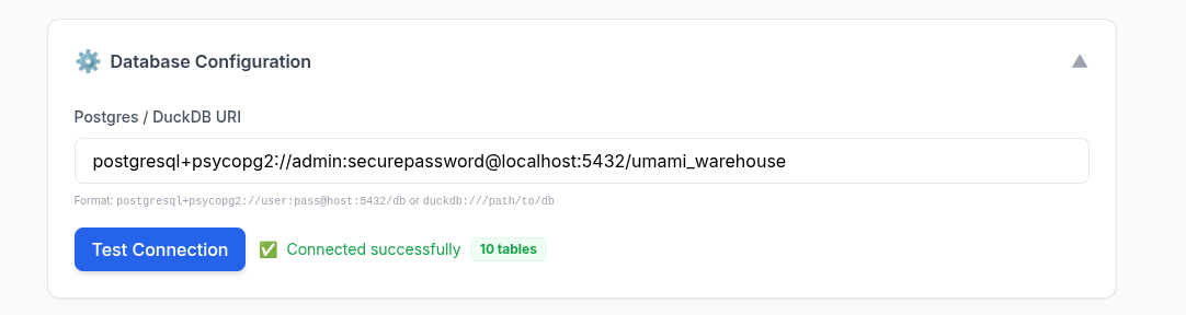
python3 baml-extract-schema.py --db-uri "postgresql://admin:securepassword@localhost:5432/umami_warehouse" --question "What are the most visited pages?"That part, BAML can take care of.
But first, a look to few popular storage for enterprises.
TSQL
Transact SQL - Tsql.
T‑SQL is Microsoft’s extended SQL dialect with procedural extras like variables, loops, and TRY…CATCH for stored procs/triggers.
Microsoft SQL Server is the RDBMS engine that runs T‑SQL (and standard SQL) for data storage/querying. T‑SQL code isn’t fully portable to other DBs like Postgres, but SQL Server is the primary platform for it. SQL Server self‑hosting is fully legal for internal/on‑premises use via Per Core/Server+CAL licenses assigned to your hardware/VMs.
Free Express/Developer editions work for small‑scale or dev; SaaS hosting needs special self‑hosted app rules or SPLA.
Oracle SQL
Oracle SQL refers to the SQL dialect used in Oracle Database, but the procedural extension is PL/SQL (Procedural Language/SQL), which is Oracle’s equivalent to T-SQL.
PL/SQL seamlessly extends standard SQL with procedural constructs like loops, conditions (IF-THEN-ELSE), exception handling, variables, procedures, functions, packages, triggers, and collections (arrays). en.wikipedia
It’s compiled and stored server-side in Oracle Database, enabling efficient data processing without app roundtrips.
DuckDB vs ClickHouse vs SQLite
Some people say that duckdb is the opposity of redshift.
The most common shorthand is: DuckDB is to Redshift (both columnar, OLAP) what SQLite is to PostgreSQL.
SQLite and DuckDB are both embedded, but they target almost opposite workloads: SQLite is for small transactional apps, DuckDB is for local analytics on larger datasets. betterstack
Mental model (when to use which)
Use SQLite when you need:
Use DuckDB when you need:
- OLAP‑style queries: big scans, joins, aggregations over millions of rows. duckdb
- Columnar / vectorized execution, parallelism, and larger‑than‑memory analytical queries. docs.kanaries
- To query Parquet/CSV files or power local analytics / BI / data‑science workflows. docs.rilldata
Architecture and performance
- Storage model: SQLite is row‑oriented, great for reading/writing whole rows quickly; DuckDB is columnar, great for scanning a few columns over many rows. betterstack
- Execution engine: SQLite processes tuples row‑by‑row; DuckDB uses columnar‑vectorized batches, which radically reduces per‑value overhead on analytical workloads. docs.kanaries
- Parallelism: SQLite uses a single thread per query and a single‑writer model; DuckDB parallelizes queries across cores and can spill to disk for out‑of‑core analytics. datacamp
- Typical result: On big analytical queries DuckDB is often orders of magnitude faster; on small indexed lookups SQLite is very competitive or better. motherduck
Practical scenarios (for your kind of projects)
Indie SaaS / web apps
- Primary OLTP DB: usually Postgres/MySQL; SQLite as a light embedded component or for single‑tenant local deployments. sqlite
- For this, DuckDB is not a replacement; it’s more a companion for analytics.
Local analytics / “Edge” or on‑device data work
- If you’re crunching logs, metrics, Parquet/CSV locally (ETL, dashboards, experiments), DuckDB is a sweet spot: embedded, but with warehouse‑like query power. linkedin
- Example: Your app writes events to files or SQLite, and a DuckDB process periodically loads them and produces aggregates.
Hybrid pattern that maps well to libSQL/Turso
- OLTP: SQLite/libSQL/libSQL‑server (like in the video) for app state and transactional behavior. sqlite
- OLAP: DuckDB reading replicated snapshots (or WAL‑derived files, or exported Parquet) for heavy analytics, without touching the hot OLTP path. motherduck
| Aspect | SQLite | DuckDB |
|---|---|---|
| Workload focus | OLTP: small, frequent reads/writes, point lookups. betterstack | OLAP: scans, joins, aggregations on large datasets. betterstack |
| Storage | Row‑based, page‑oriented. betterstack | Columnar storage. betterstack |
| Execution | Tuple‑at‑a‑time, single‑threaded per query. betterstack | Columnar‑vectorized, multi‑core parallel. betterstack |
| Best use cases | Embedded app DB, config, cache, mobile/IoT, small web backends. datacamp | Local analytics, data science, BI, ETL over Parquet/CSV/SQLite dumps. datacamp |
| Scalability style | Scales in simplicity and deployment ubiquity; limited for heavy analytics and concurrency. datacamp | Scales in analytical throughput, can handle larger‑than‑memory datasets via out‑of‑core execution. datacamp |
ClickHouse, DuckDB, and SQLite form a nice spectrum: SQLite for embedded OLTP, DuckDB for local OLAP in‑process, ClickHouse for large, multi‑user OLAP clusters. airbyte
Mental model in one line each
- SQLite: Tiny, embeddable transactional store for apps (phones, desktop, IoT, small web backends). betterstack
- DuckDB: Embeddable analytical engine for local, in‑process queries over files or small/medium datasets. datacamp
- ClickHouse: Distributed columnar OLAP database for large‑scale, real‑time analytics and dashboards. influxdata
Core roles
SQLite
- OLTP focus: fast inserts/updates, point lookups, simple queries. betterstack
- Row‑based storage, single‑file deployment, minimal footprint. datacamp
- Great for configs, local data, offline‑first apps, small SaaS backends. datacamp
DuckDB
- OLAP focus: scans, joins, aggregations on millions of rows. duckdb
- Columnar + vectorized engine, optimized for running inside your app / notebook. influxdata
- Ideal for data‑science workflows, querying Parquet/CSV, interactive local analytics. docs.rilldata
ClickHouse
Choose SQLite when:
- You’re building a small web/desktop/mobile app and need a simple, reliable embedded DB. betterstack
- Data volume is modest, queries are simple, and you care about minimal ops and footprint. betterstack
Choose DuckDB when:
Choose ClickHouse when:
- You need multi‑user analytics over very large, fast‑growing datasets (events, observability, billing, recommendations). gocodeo
- You want real‑time dashboards and complex queries with low latency at high concurrency. instaclustr
Architectural fit examples
Indie SaaS with analytics inside the product
Analytics platform / observability tool
Side‑by‑side overview
| Aspect | SQLite | DuckDB | ClickHouse |
|---|---|---|---|
| Primary workload | OLTP (app data, configs, caches). betterstack | OLAP (local analytics, ETL, data science). betterstack | OLAP (large‑scale, real‑time analytics). airbyte |
| Deployment | Embedded library, single file on disk. betterstack | Embedded, in‑process; no server. betterstack | Server/cluster, distributed nodes. airbyte |
| Storage model | Row‑based. betterstack | Columnar. betterstack | Columnar. airbyte |
| Scale sweet spot | MB–few GB, single‑user/small multi‑user. betterstack | GB–tens/hundreds of GB on one machine. datacamp | Hundreds of GB–TB+ across many nodes. airbyte |
| Typical use | App DB, offline storage. betterstack | Notebook/ETL analytics, local dashboards. datacamp | Logging, metrics, product analytics, BI. airbyte |
This is where it all connects in the D&A space:
mindmap
  root((Data Modeling))
    OLTP
      [Process: Transactional]
      Concept: ER Modeling
        )Normalized - 3NF(
        Goal: Data Integrity
        Low Redundancy
      Characteristics
        ACID Compliance
        Row-based Storage
        High Write Speed
        Low Latency - ms
      Tools
        PostgreSQL
        MySQL
        MariaDB
        SQLite
    OLAP
      [Process: Analytical]
      Concept: Dimensional Modeling
        )Star / Snowflake Schema(
        Goal: Query Performance
        High Redundancy
      Characteristics
        Fact & Dimension Tables
        Columnar Storage
        High Read Speed
        Complex Aggregations
      Tools
        ClickHouse
        DuckDB - Local
        Snowflake
        BigQuery
    The Bridge
      ))ETL / ELT((
      )Data Warehouse(
The Data Lakehouse is essentially the “modern evolution” that tries to delete the line between your Postgres (OLTP) and your ClickHouse/DuckDB (OLAP).
If OLTP is for writing and OLAP is for reading, the Lakehouse is for unifying.
mindmap
  root((Data Management))
    OLTP (Postgres/MariaDB)
      ::icon(fa fa-database)
      Focus: Live Transactions
      Format: Row-based tables

    OLAP (DuckDB/ClickHouse)
      ::icon(fa fa-chart-line)
      Focus: Fast Analytics
      Format: Memory/Columnar

    Data Lakehouse (The Hybrid)
      Concept: Best of both worlds
      Architecture
        Object Storage (S3/MinIO)
        Table Formats (Delta Lake/Iceberg)
      File Formats (The "Big Data" part)
        Avro: Fast Write/Streaming
        Parquet: Fast Read/Analytics
      Key Benefits
        ACID on top of Files
        One single source of truth
        Cheaper than Warehouse
Using BAML
I was testing BAML last year here.
Its not as popular as langchain, but still: https://github.com/BoundaryML/baml

Tt resonated a lot with the way langchain generates the query to the databases.
So could not resist to explore how to do a custom and more controlable solution around BAML.
![]()
What I wanted is this: and remove the langchain dependency
- Extract Schema: Use
SQLDatabaseto get the metadata. - Generate & Separate: Call BAML and extract the three distinct fields (
sql,explanation,promptRationale). - Execute: Run the query against the DB using the existing connection.
- Final Output:
- Print the Rationale (Why we did this).
- Print the SQL (What we are running).
- Print the Data Table (The results).
./datachat_venv/bin/baml-cli generate --from z-langchain2baml/baml_srcgraph LR
U[User Question] --> S[Python Script]
S --> |Conn| DB[(PostgreSQL)]
DB --> |Full Schema| S
S --> |Context + Question| B[BAML Client]
B --> |Prompt| L[LLM GPT-4o]
L --> |JSON Result| B
B --> |Typed Object| S
S --> Out[Final SQL & Explanation]
Out --> DB
DB --> Result[Data Result]
Result --> S- Activate Environment:
source datachat_venv/bin/activate
#pip install tabulate- ReCreate baml arficats:
baml-cli init #configure your baml_src
baml-cli generate #it generates baml_client, which the main python script uses
Working with BAML follows a very specific and reliable cycle:
- Define (
baml_src/): You define your data models (classes) and functions in.bamlfiles.database.baml: Defines theSqlResultstructure and theGenerateSQLfunction.clients.baml: Configures the LLM providers (e.g., GPT-4o).
- Generate (
baml_client/): Runningbaml-cli generateturns your BAML definitions into a type-safe Python client. You never edit this folder manually. - Call (Python): Your application script (
baml-qna.py) imports the generated client and calls the functions just like regular Python methods.
How to Tweak the Logic (baml_src/)
If you want to customize the behavior, here is what each file does:
database.baml: The Core Logic. This is where you define theclass(what data the LLM returns) and thefunction(the actual prompt). If you want to change how the LLM thinks or what info it provides, edit this.clients.baml: The Model Settings. Here you define which LLM providers to use (OpenAI, Anthropic, etc.), which models (GPT-4o, Claude 3.5), and parameters liketemperatureorapi_keyenvironment variables.generators.baml: The Integration Settings. This tells BAML to generate a Python client and where to put it. You rarely need to touch this unless you are switching languages or changing the output path.
graph LR
    Start([Start]) --> Init[baml-cli init]
    Init --> Src[baml_src folder]
    Src --> Edit[Edit .baml files]
    Edit --> Gen[baml-cli generate]
    Gen --> Client[baml_client folder]
    Client --> Py[Python Script]
    Py --> Call[Client Calls LLM]

    subgraph "Manual Input"
    Edit
    end

    subgraph "Auto-Generated"
    Client
end- Run Execution Script: provide your local pgsql connection
# From the project root
python3 z-langchain2baml/baml-qna.py --db-uri "postgresql://admin:securepassword@localhost:5432/umami_warehouse" --question "What are the most visited pages?"
By separating promptRationale, we gain:
- Debugging: Understand if the LLM misinterpreted the schema.
- Auditing: Keep track of why certain joins or filters were applied.
- User Trust: Show the user the “thinking process” before showing the data.
mindmap
  root((baml-qna.py))
    BAML
      Structured Output
      Type-safe Python Client
      Prompts & Schema Context
      Model Clients (GPT-4o)
    PostgreSQL
      Data Warehouse
      Schema Metadata source
      SQL Execution target
    General Python Logic
      Orchestration
      LangChain: Schema Extraction
      Pandas: Data Result Formatting
      SQLAlchemy: DB Connection
UI Wrapper
To make the solution sellable to enterprises: we need a UI.
And the good news is that we already vibe coded that: here.
Even with a related tech talk
Well, Ok.
Not only a UI, but a way to get plots and potentially dashboards done from natural language.
Or as people call this now: a generative BI solution.
Thats coming up next: z-baml-genbi
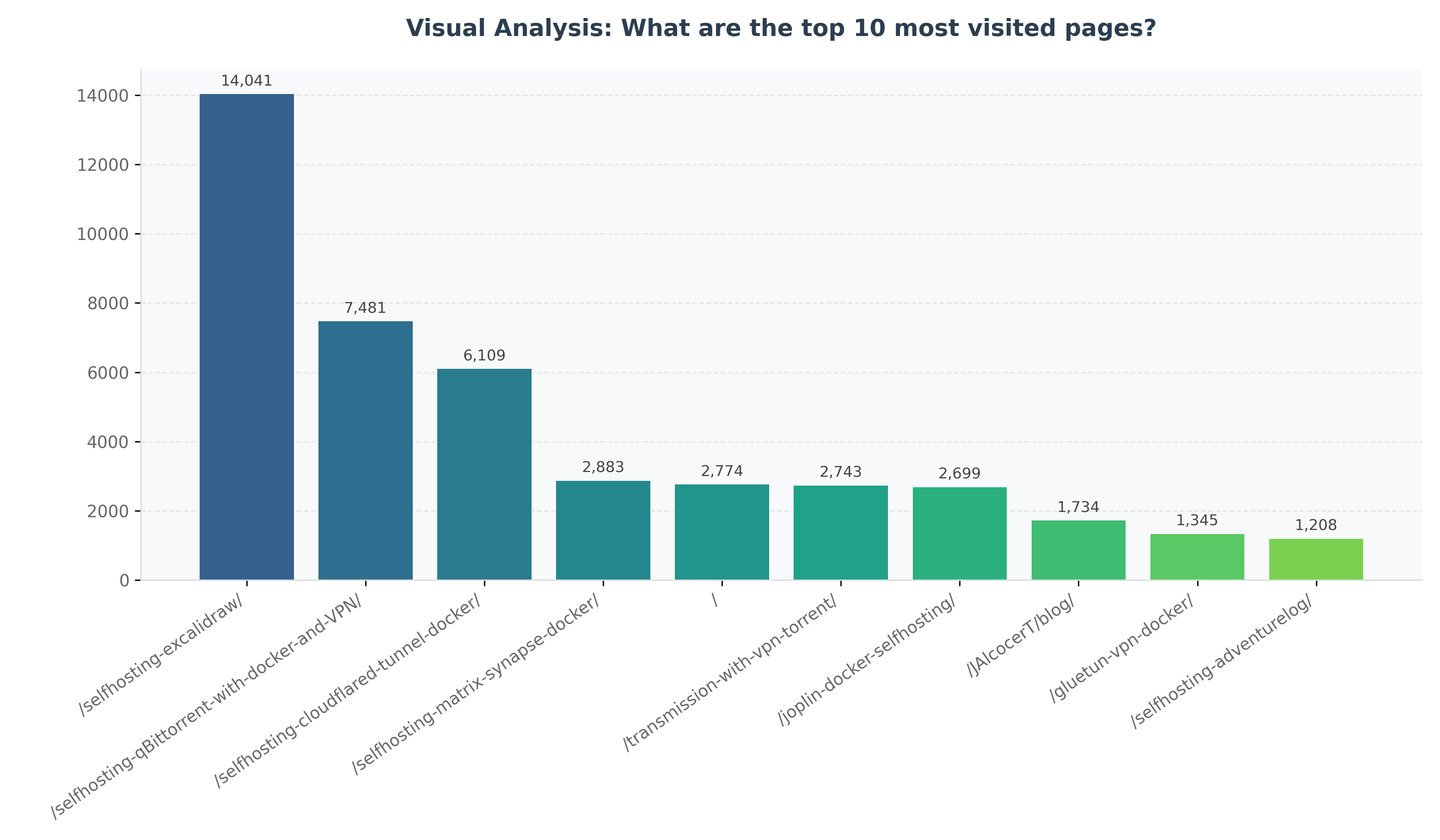
Imagine having such graphs generated directly from your QnA. No SQL, No dashboarding.
Conclusions
Another example of how we are moving From how to what and why.
Code is cheap now. Software isnt at least for now.
From this great post and video
The danger is now more on not to get distracted with the daily tool or workflow that gets released.
Go with whatever: cursor, antigravity, claude code, lovable, opencode, crush…
But just go and try.
The challenge is now the distribution / orchestration / marketing, which are other OpEx, not the coding thing.
Do you even know the audience? is it even listening?
Are you building sth for an empty room?
Time to go from builder to creator and finding people to care about your thing.
The related tech talk
If there was any doubt, if put together a ppt, taking into consideration these engagement points:
git clone https://github.com/JAlcocerT/selfhosted-landing
cd y2026-tech-talks/4-baml-db-insightsFAQ
A Recap on D&A for Interviews
- Document Logic (The Planning)
- BRD (Business Requirements): Answers “WHY build this?” (The Vision & Goals).
- PRD (Product Requirements): Answers “WHAT are we building?” (The Features & Roadmap).
- FRD (Functional Requirements): Answers “HOW does it work?” (The Technical Logic & CRUDs).
- Data Logic (The Analytics)
- Fact Tables: Answer “WHAT happened (and how much)?”
- Examples:
visit_count,revenue,quantity_sold.
- Examples:
- Dimension Tables: Answer “WHO / WHERE / WHICH context?”
- Examples:
customer_name,product_category,country_origin.
- Examples:
If you were to grow your Northwind project into a “Big Data” architecture:
Postgres (OLTP) handles your orders.
An ETL tool takes those orders and saves them as Avro files in a folder (Data Lake).
A “Lakehouse” tool (like Apache Iceberg or Delta Lake) converts those to Parquet.
DuckDB or ClickHouse then queries those Parquet files directly.
| Aspect | Dimensional Modeling | Semantic Modeling (PBI) |
|---|---|---|
| Focus | Efficiency and Structure (Star Schema). | Usability and Business Logic (Logic + Context). |
| Action | Joining tables, defining PKs and FKs. | Refinement: DAX, Renaming, RLS, Formatting. |
| Output | A clean, technical Warehouse schema. | A “Self-Service” model ready for business users. |
The Traditional BI Lifecycle (Hand-Crafted)
To demonstrate the value of Gen-BI, we must first understand the manual effort required to build a high-performance Power BI dashboard aligned with business goals.
The Bridge from Raw Data to Insights
Building a professional Power BI solution involves a rigorous 4-step process:
- Data Acquisition (DL - Data Layer): Connecting to raw sources via SQL or Power Query. This is where the physical connection lives.
- Dimensional Modeling (The Foundation): Implementing Kimball Methodology.
- Creating a Star Schema with clear
Facttables (events) andDimensiontables (attributes). - This is the “Structural Truth” of the data.
- Creating a Star Schema with clear
- Semantic Modeling (The Meaning): Adding the Power BI Layer.
- Writing DAX Measures (e.g., Year-to-Date, Moving Averages).
- Setting up Hierarchies (e.g., Category -> Product).
- Optimizing performance via Aggregations and Column indexing.
- Visualization (RL): Aligning with the Business Purpose.
- Selecting visuals that answer specific BRD questions (e.g., “Which region is underperforming?”).
- Tuning the UX for speed and clarity.
Document Logic (The Planning):
- BRD (Business Requirements): Answers “WHY build this?” (The Vision & Goals).
- PRD (Product Requirements): Answers “WHAT are we building?” (The Features & Roadmap).
- FRD (Functional Requirements): Answers “HOW does it work?” (The Technical Logic & CRUDs).
Data Logic (The Analytics):
- Fact Tables: Answer “WHAT happened (and how much)?”
- Examples: visit_count, revenue, quantity_sold.
- Dimension Tables: Answer “WHO / WHERE / WHICH context?”
- Examples: customer_name, product_category, country_origin.
In the world of data engineering, these concepts form the fundamental “fork in the road” between how we store data for action versus how we store it for analysis.
- OLTP: The “Action” Layer
OLTP (Online Transaction Processing) systems are built to handle the daily operations of a business (e.g., swiping a credit card, updating a password, or placing an order).
- Mapping: ER Modeling Normalization
- The Goal: Data Integrity. You want to ensure that if a customer changes their address, you only have to update it in one place.
- Why Normalization? By breaking data into many small, related tables (usually 3rd Normal Form), you eliminate redundancy. This makes “writes” (INSERT, UPDATE, DELETE) lightning-fast and prevents data anomalies.
- OLAP: The “Analysis” Layer
OLAP (Online Analytical Processing) systems are built for complex decision-making (e.g., “What were our total sales in the Northeast region vs. the Southwest over the last three years?”).
- Mapping: Dimensional Modeling Denormalization
- The Goal: Query Performance & Simplicity. Analysts don’t want to join 50 tables to get one report. They want the data pre-organized for speed.
- Why Denormalization? You intentionally bring data back together. While this creates “redundancy” (the same city name might appear 1,000 times), it drastically reduces the number of “joins” the database has to perform, making “reads” much faster.
- Star vs. Snowflake (The OLAP Variations)
Within Dimensional Modeling, you have two primary ways to structure your “Dimensions”:
| Feature | Star Schema (Most Common) | Snowflake Schema |
|---|---|---|
| Structure | Denormalized. Dimension tables are flat. | Normalized. Dimension tables are broken down further. |
| Visual | Looks like a star (Fact table in the center). | Looks like a snowflake (Dimensions have sub-dimensions). |
| Performance | Faster. Fewer joins required. | Slower. More joins required. |
| Maintenance | Harder; data redundancy is high. | Easier; less redundancy (easier to update a category name). |
| System Type | Modeling Style | Strategy | Focus |
|---|---|---|---|
| OLTP | Entity-Relationship (ER) | Normalization | Fast Writes / Data Integrity |
| OLAP | Dimensional | Denormalization | Fast Reads / Easy Analysis |
The best way to see the difference between Lloyd Tabb’s Looker and Microsoft’s Power BI is to look at how they handle a simple request: “Calculate our Gross Profit Margin.”
1. The Power BI Way (DAX)
In Power BI, you write a Measure. This is a formula that lives inside your report file. It looks very similar to an advanced Excel formula.
The Code (DAX):
Gross Profit Margin =
DIVIDE(
    SUM(Sales[Revenue]) - SUM(Sales[Cost]),
    SUM(Sales[Revenue]),
    0
)- Where it lives: Inside a specific
.pbixfile or a specific dataset. - The User Experience: A user drags this “Measure” onto a chart. If they want to see it by “Year,” Power BI recalculates that formula for every year on the fly.
- The Problem: If another analyst creates a different report and writes
(Total_Rev - Total_Cost) / Total_Revmanually, and forgets to handle the “divide by zero” error, your company now has two different versions of the same metric.
2. The Looker Way (LookML)
In Looker, you don’t write a formula for a specific report. You define the Logic in a central code file called LookML.
The Code (LookML):
view: orders {
  sql_table_name: production.orders ;;

  measure: total_revenue {
    type: sum
    sql: ${TABLE}.revenue ;;
  }

  measure: total_cost {
    type: sum
    sql: ${TABLE}.cost ;;
  }

  measure: gross_profit_margin {
    type: number
    sql: (${total_revenue} - ${total_cost}) / NULLIF(${total_revenue}, 0) ;;
    value_format_name: percent_2
  }
}- Where it lives: In a centralized Git repository (like GitHub).
- The User Experience: The business user never sees this code. They just see a button labeled “Gross Profit Margin” in a browser.
- The Benefit: Because the logic is defined in one central place, it is impossible for two people to have different “Profit Margin” numbers. If you update the code, every dashboard in the entire company updates instantly.
Summary of the Difference
| Feature | Power BI (DAX) | Looker (LookML) |
|---|---|---|
| Vibe | “Supercharged Excel” | “Software Engineering for Data” |
| Logic Location | Often scattered across many reports. | Strictly centralized in one “Model.” |
| Version Control | Hard (saving versions of files). | Native (Integrated with Git/GitHub). |
| Data Movement | Usually “Imports” data into its own RAM. | Never moves data. Always queries your database (Redshift/Postgres) live. |
Lloyd Tabb’s big “Aha!” moment was realizing that data analysts should act more like software engineers—writing reusable, version-controlled code rather than building one-off spreadsheets.
To understand semantic modeling in Power BI, it helps to think of it as the “Translation Layer.”
While Dimensional Modeling is about how you organize data in the warehouse, Semantic Modeling is about how you present that data to humans.
- Semantic vs. Dimensional Modeling
| Feature | Dimensional Modeling (The Foundation) | Semantic Modeling (The Interface) |
|---|---|---|
| Objective | Organizing data for performance and storage. | Organizing data for business logic and usability. |
| Common Shapes | Star Schema, Snowflake Schema. | Power BI Datasets, Looker LookML, Metrics Layer. |
| Key Components | Facts (Numbers) and Dimensions (Attributes). | Measures (DAX), Hierarchies, Relationships, Metadata. |
| Analogy | The way books are categorized and stored on library shelves. | The searchable digital catalog that helps you find and understand the books. |
- Approaches to Semantic Modeling in Power BI
There are three main “architectural” ways to handle this in the Microsoft ecosystem:
A. The “Golden Dataset” Approach (Centralized)
You create one single, highly polished Power BI file (.pbix) that contains the Star Schema, all DAX measures, and row-level security.
- How it works: You publish this to the Power BI Service. Other users then “Connect to Power BI Dataset” to build their own reports.
- Pro: One single source of truth.
- Con: Can become a bottleneck if one person manages the “Golden” model for the whole company.
B. The “Composite Model” Approach (Hybrid)
This allows you to connect to a “Golden Dataset” but also add your own local data (like an Excel file or a specific SQL table) on top of it.
- How it works: It uses “DirectQuery for Power BI datasets.”
- Pro: Flexibility for departments to customize data without breaking the central logic.
- Con: Can become complex to manage and slightly slower in performance.
C. The “External” Semantic Layer (Headless BI)
Instead of defining logic inside Power BI, you define it in a tool that sits between your warehouse (Redshift/Snowflake) and Power BI.
- Examples: dbt Semantic Layer, Cube, or AtScale.
- How it works: You write your metrics in YAML or SQL. Power BI connects to these tools as if they were a database.
- Pro: If you switch from Power BI to Tableau or Looker, your metrics stay exactly the same.
- How to “Do” Semantic Modeling Right
Regardless of the approach, follow these rules to ensure your Power BI model is “Semantic”:
- Hide the Plumbing: Hide all Foreign Key columns (the IDs used for joins). Users should only see descriptive names like “Product Name,” not
FK_Prod_ID_99. - Explicit Measures: Never let users “Auto-Sum” a column. Create an explicit DAX measure:
Total Sales = SUM(Sales[Amount]). This ensures the calculation is the same everywhere. - Folders and Descriptions: Use “Display Folders” to group measures (e.g., “Time Intelligence,” “Profitability”) and add descriptions to fields so users see a tooltip explaining what the data means.
- Hierarchies: Create “Drill-down” paths (Country > State > City) so the model feels intuitive to browse.
If you are coming from the Lloyd Tabb/Looker world, Power BI feels different because the “Semantic” part is often bundled inside the report file. However, by using Power BI Datasets (Live Connection), you can replicate that “Looker Vibe” where the logic is centralized and separated from the visuals.
SQL vs Malloy
Malloy is a modern, open-source language for data modeling and querying, created by Lloyd Tabb (the founder of Looker) and a team at Google.
MIT | Malloy is a modern open source language for describing data relationships and transformations.
If LookML was Lloyd Tabb’s first attempt to fix SQL, Malloy is his “clean slate” version.
It is designed to be for SQL what TypeScript is for JavaScript:
A more powerful, typed, and modular way to write code that ultimately “compiles” down to standard SQL.
What makes Malloy special?
- “Escaping the Rectangle”
Standard SQL forces data into “rectangles” (rows and columns). If you want to see an Order and all its Items, you have to “flatten” the data, which leads to duplicate rows and complex JOIN logic.
- Malloy’s Fix: It natively handles nested data and hierarchies. You can query a “Table within a Table” naturally, which makes it much easier to build dashboards that show a summary and a breakdown in the same view.
- Reusable “Measures” (The Semantic Part)
In SQL, if you want to calculate “Gross Margin,” you have to write that math in every single query.
- Malloy’s Fix: You define
gross_marginonce in the model. From then on, you just reference it. If the definition changes, you update one line of code, and every query using it is fixed.
- Automatic “Symmetric Aggregates”
One of the most dangerous things in SQL is the “Fan-out” (doubling your totals because of a Join).
- Malloy’s Fix: It has built-in logic that understands the relationships between tables. It automatically prevents “double counting” when you join a one-to-many relationship, so your sums are always correct without you needing to worry about
DISTINCThacks.
| Feature | SQL | Malloy |
|---|---|---|
| Logic | Imperative (You tell it how to join/group). | Declarative (You tell it what you want). |
| Reusability | Low (Copy-paste logic). | High (Define once, use everywhere). |
| Complexity | 100 lines for a nested report. | 10 lines for the same report. |
| Output | Rectangles only. | Nested/Hierarchical JSON or Tables. |
How to use it: because Malloy isn’t a database itself.
It is a compiler.
You write Malloy code, and it converts it into optimized SQL for:
- DuckDB (Native support, great for local Parquet files).
- BigQuery.
- PostgreSQL.
- Snowflake.
Is it still “Experimental”?
As of late 2023, the team released Malloy 4.0, which they officially called the “end of the experimental phase.”
It is now considered a stable, open-source language that is ready for production use, primarily through their excellent VS Code Extension.
Comparing Malloy to DuckDB, SQLite, ClickHouse, and Redshift is a bit like comparing a GPS system to different types of Engines.
Malloy is the Language/Interface (the GPS), while the others are the Databases/Engines (the car). You need one of each to actually “drive” your data.
- The Big Distinction: Language vs. Engine
| Tool | Category | What it does |
|---|---|---|
| Malloy | Modeling Language | Compiles into SQL. It’s a “wrapper” that makes querying easier and reusable. |
| DuckDB | Embedded OLAP DB | A fast, local engine for analyzing files (Parquet/CSV) on your laptop. |
| SQLite | Embedded OLTP DB | A lightweight engine for apps/storage. Great for writing, slow for big analysis. |
| ClickHouse | Distributed OLAP DB | A massive, server-based engine for real-time analytics on billions of rows. |
| Redshift | Cloud Data Warehouse | Amazon’s enterprise-scale engine for massive, long-term data storage. |
- How Malloy interacts with them
Malloy doesn’t store data.
It connects to these engines and tells them what to do.
- Malloy + DuckDB: The most common “modern” combo. You use Malloy to write clean code, and DuckDB executes it instantly on your local files.
- Malloy + Redshift: Malloy replaces the “messy” SQL you would normally send to Redshift, making your enterprise queries shorter and more readable.
- Malloy + ClickHouse: Currently, Malloy has limited/community support for ClickHouse (it primarily focuses on BigQuery, Postgres, and DuckDB), but the logic is the same: Malloy writes the SQL so you don’t have to.
- Comparing the “Engines” (The Databases)
| Feature | SQLite | DuckDB | ClickHouse | Redshift |
|---|---|---|---|---|
| Best For | Mobile apps, local storage. | Data Science, local Parquet. | Real-time web analytics. | Enterprise BI. |
| Modeling | ER (Row-based) | Dimensional (Column) | Dimensional (Column) | Dimensional (Column) |
| Scale | Megabytes to Gigabytes. | Gigabytes (Single Node). | Terabytes to Petabytes. | Petabytes (Cloud). |
| Speed | Fast for 1 row. | Fast for 1M rows. | Fast for 1B rows. | Fast for complex Joins. |
- Which one should you use for your project?
If you are following the Lloyd Tabb philosophy:
- Use DuckDB as your engine if you want to play with your Northwind data locally on your computer. It’s free and requires zero setup.
- Use Malloy as your language on top of DuckDB. This will allow you to define your “Gross Profit” or “Total Orders” logic once and reuse it across every chart.
- Avoid SQLite for this specific task—it’s a great database, but it will struggle once you start doing the “Nested” and “Complex” analytical queries that Malloy is designed for.
Summary
- Malloy is the Smart Translator (created by the Looker founder). https://www.youtube.com/watch?v=pLeF4j_Irg4
- DuckDB is the Local Turbo-Engine.
- ClickHouse/Redshift are the Industrial Power-Plants.
A great video about Apache Iceberg:
Apache Kafka:
A Materialized table is a solution to a d&a problem.
A Materialized View is essentially a “cached” table. While a regular view is just a saved SQL query that runs every time you look at it, a materialized view calculates the result once and stores it physically on the disk as a real table.
Think of it like this:
- Regular View: A recipe. Every time you want a cake, you have to follow the recipe and bake it from scratch. (Fresh, but slow).
- Materialized View: A pre-baked cake. When you want a cake, you just grab it from the fridge. (Instant, but might be a day old).
Why is it useful?
- Speed (Performance): If your query joins 10 huge tables and takes 2 minutes to run, a materialized view runs it once (e.g., at 3 AM) and saves the result. When you query the view at 10 AM, it’s nearly instantaneous.
- Saves Money/Compute: You aren’t paying your database (like Snowflake or BigQuery) to recalculate the same complex math 100 times a day.
- Simplicity: It hides complex “Big Data” messiness. Your data analysts just see a clean, fast table.
Do Power BI or Looker have them?
Technically, “Materialized View” is a database feature (Postgres, BigQuery, Snowflake, etc.), but both Power BI and Looker have their own versions to achieve the same result.
1. Looker: Persistent Derived Tables (PDTs)
Looker doesn’t call them materialized views; it calls them PDTs.
- How it works: You write the SQL for a table in LookML. Looker then creates a physical table in your database (e.g., Redshift or BigQuery) and updates it on a schedule.
- Refinement: Looker can even do “Incremental PDTs” where it only adds the newest rows instead of rebuilding the whole thing.
2. Power BI: Calculated Tables / Aggregations
Power BI handles this slightly differently depending on your setup:
- Import Mode: When you “Import” data, the entire dataset is essentially a materialized view. It’s stored in Power BI’s memory.
- Calculated Tables: You can use DAX to create a new table based on others. This table is “materialized” inside the Power BI file during the refresh.
- User-Defined Aggregations: You can tell Power BI to create a hidden, summarized version of a huge “DirectQuery” table. When a user asks for a high-level chart (e.g., “Sales by Year”), Power BI hits the “materialized” summary instead of the billion-row table.
Summary Comparison
| Tool | Feature Name | Stored In… |
|---|---|---|
| Database (e.g., Postgres) | Materialized View | The database disk. |
| Looker | Persistent Derived Table (PDT) | The database disk (managed by Looker). |
| Power BI | Calculated Table / Aggregation | Power BI’s internal Memory/Cache. |
When to use one?
- Use a Regular View if your data changes every second (real-time) and the query is simple/fast.
- Use a Materialized View (or PDT) if you have a massive dataset and your dashboards are starting to feel slow or “laggy.”
PGSQL vs The Rest
PGSQl vs RedShift
The short answer is: No, Redshift is not “Serverless PostgreSQL.” While Amazon Redshift was originally based on an older version of PostgreSQL (8.0.2), it has evolved into a fundamentally different animal designed for a completely different purpose.
To help clarify, here is how the two compare and where they fit in your tech stack:
- Architectural Differences
The most critical difference is how they store and process data.
- PostgreSQL (Row-oriented): Designed for OLTP (Online Transactional Processing). It stores data in rows, which is perfect for small, frequent operations like “Update this user’s email” or “Insert a new order.”
- Redshift (Column-oriented): Designed for OLAP (Online Analytical Processing). It stores data in columns, which is vastly superior for scanning massive datasets to find trends, such as “What was the average revenue per month for the last five years?”
| Feature | PostgreSQL | Amazon Redshift |
|---|---|---|
| Primary Use | App backend, transactions | Data warehousing, big data analytics |
| Storage Type | Row-based | Column-based |
| Scaling | Vertical (bigger servers) | Horizontal (more nodes in a cluster) |
| Integrations | General purpose | Deeply integrated with AWS (S3, Glue, etc.) |
- Is it Serverless?
Amazon offers a product called Redshift Serverless, which allows you to run analytical queries without managing clusters or nodes. However, this is still a Data Warehouse, not a general-purpose transactional database.
If you are looking for a Serverless PostgreSQL, the actual AWS equivalent is Amazon Aurora Serverless.
- The “PostgreSQL” Connection
Redshift still feels like Postgres in a few ways:
- Interface: You can use standard Postgres JDBC/ODBC drivers to connect to it.
- Syntax: Many SQL commands are the same, though Redshift has removed many Postgres features (like triggers, indexes, and certain constraints) that don’t make sense for a massive data warehouse.
- Tooling: Most BI tools that support Postgres can also connect to Redshift.
What should you use?
- Use Aurora Serverless (PostgreSQL) if you are building an app or a website and want a database that scales up and down based on user traffic.
- Use Redshift Serverless if you have millions/billions of rows of data and need to run complex analytical reports or “big data” queries.
Neon vs D1
It is helpful to think of Neon and Cloudflare D1 as competitors in the “Serverless SQL” space, but they aren’t both PostgreSQL.
Here is the breakdown of how they compare to each other and to Redshift:
- Neon: The True “Serverless Postgres”
Neon is a direct competitor to Amazon Aurora Serverless.
It is 100% PostgreSQL-compatible because it literally runs the Postgres engine, but it has a custom-built storage layer that allows it to “scale to zero” (shut down when not in use) and scale up instantly when a request comes in.
- Best for: Application backends, SaaS products, and development environments.
- Key Feature: Branching. You can “branch” your database like a Git repo, creating a perfect copy of your production data for testing in seconds.
- Cloudflare D1: The SQLite Alternative
Cloudflare D1 is not PostgreSQL—it is built on SQLite.
While it is a “competitor” to Neon in the sense that it provides a serverless database for web developers, the underlying technology is different.
- Best for: Developers already using Cloudflare Workers. It is designed to be geographically close to your users (at the “edge”).
- The Trade-off: SQLite has a different SQL dialect than Postgres. If your app relies on Postgres-specific features (like JSONB or specific extensions), you can’t easily switch to D1.
Comparison Table
| Feature | Neon | Cloudflare D1 | Amazon Redshift |
|---|---|---|---|
| Engine | PostgreSQL | SQLite | Redshift (Postgres-derivative) |
| Type | Transactional (OLTP) | Transactional (OLTP) | Analytical (OLAP) |
| Serverless? | Yes | Yes | Yes (Redshift Serverless) |
| Scale to Zero? | Yes (saves money) | Yes | Yes |
| Ideal Data Size | GBs to TBs | Small (current limit ~10GB) | TBs to PBs |
Are they Redshift competitors?
Generally, no. * Neon and Cloudflare D1 are built for speedy, small operations (e.g., “Log this user in,” “Show this profile”).
- Redshift is built for massive, heavy lifting (e.g., “Calculate total revenue across 1 billion rows for the last 3 years”).
If you tried to run Redshift-style “Big Data” queries on Neon, it would get very expensive and likely slow down.
Conversely, if you tried to use Redshift as your website’s primary database for user logins, your site would feel sluggish because Redshift isn’t optimized for millisecond-fast individual row lookups.
Which one should you choose?
- Choose Neon if you want a powerful, modern PostgreSQL experience without managing servers.
- Choose Cloudflare D1 if you are already in the Cloudflare ecosystem and need a simple, fast SQL database for a global app.
- Choose Redshift if you are doing Data Science or building a Business Intelligence dashboard.
More about BAML
BAML and function calling
BAML is a framework/DSL that treats LLM prompts as functions with typed inputs and typed outputs, compiling them into regular code (TS, Python, etc.).[1][2]
OpenAI “function calling” (tools) lets you describe functions via JSON schemas so the model can return structured JSON that you then execute in your app.[3][4]
How BAML implements LLM functions
- In BAML you write definitions like
function ExtractResume(text: string) -> Resume { ... }and BAML generates client bindings plus a prompt that injects the output schema via{{ ctx.output_format }}.[5][2] - It uses Schema‑Aligned Parsing (SAP) to repair and coerce the model’s output into the target schema quickly, improving reliability over raw JSON parsing.[6][5]
How OpenAI function calling works
- You pass a
toolsarray describing your functions (name, description, JSON parameter schema) and the model responds with tool calls plus arguments in JSON when appropriate.[4][3] - Your code parses those arguments, calls your real functions or APIs, optionally feeds results back to the model, and continues until you have a final answer.[3]
Routing to Astro components
- Both approaches can be used as a “router” layer: the LLM chooses among logical actions like
show_homepage,show_product({ slug }), etc., and your Astro server code maps those actions to pages/components.[7][8] - With OpenAI tools you expose these as functions; with BAML you might define a single
RouteQuery(query) -> RouteDecisionunion type and switch on that to choose the Astro route.[9][5]
Practical upshot for your use case
- Yes, either OpenAI function calling or BAML can decide which Astro component/page to serve based on a user’s query; the difference is mostly ergonomics and robustness of structured output.
BAML gives you stronger typing and parsing; OpenAI tools are simpler if you’re already in that ecosystem.
LibSQL?
This come from a YouTube video titled “The Inevitable Evolution of SQLite” from the DevOps Toolbox series, published on Jan 16, 2026, about an 11‑minute overview of libSQL and related tooling.
- Presents libSQL as an open‑source fork of SQLite that accepts external contributions and is designed for replication, distribution, and scale.
- Shows LibSQL server (sqld) providing remote access similar to PostgreSQL/MySQL, with a core in C and new server features in Rust.
- Mentions Turso’s in‑progress Rust rewrite (Torso, previously Limbo) as “next evolution of SQLite,” but that is left for another video.
Key ideas about SQLite vs libSQL
- SQLite’s limitations called out: it is a single file on disk that is great for many workloads but not straightforward to cluster, shard, or distribute.
- libSQL adds replication, remote access, vector types, and nicer CLIs on top of SQLite semantics while still relying on a WAL file for write‑ahead logging and data integrity.