Suspension videos
Tl;DR
Intro
- WHY Im writting this post:
- What Ive learnt with it: Ive ended
Some months ago, cc 4.6 was not there for engine balance
MBSD OSS Fwk
Ive been following this roadmap, to get couple of fully OSS MIT licensed repos out there:
So what?
You can now:
Via the web https://github.com/JAlcocerT/multi-body
Suspensions Types
Suspension Modelling
Quarter car


Half car
- Suspensions: Double Wishbone, macpherson…
https://www.youtube.com/shorts/cx21pJaPVTc
Suspension design space
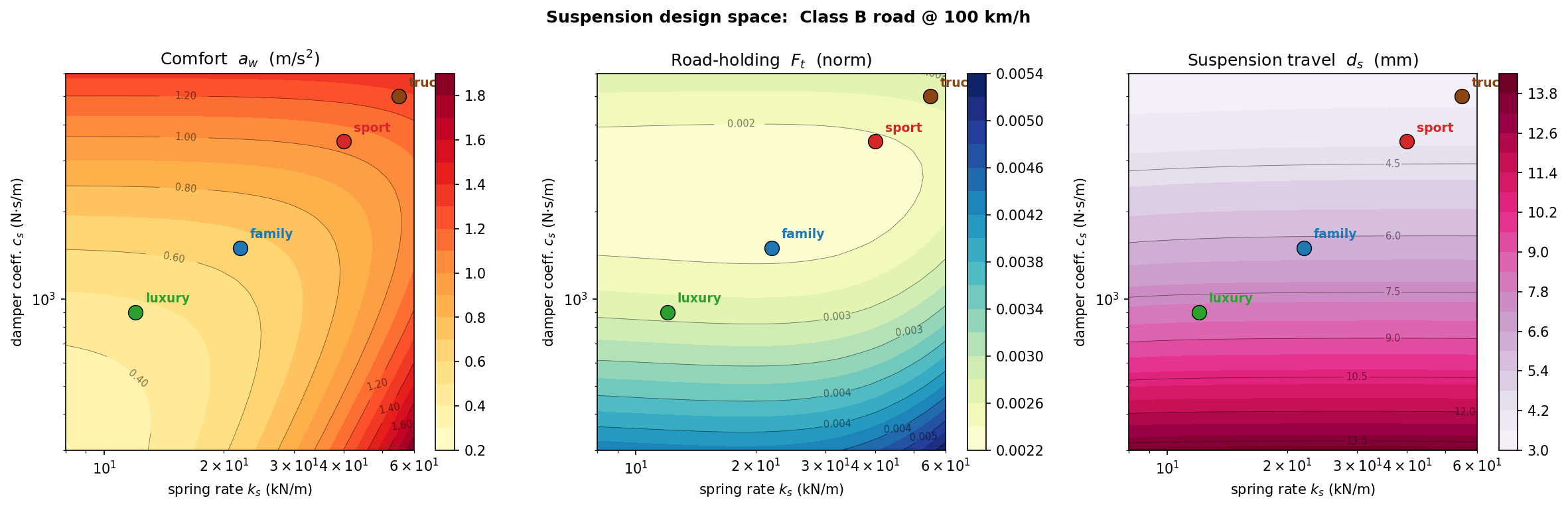
This chapter provides the “Engineering Conclusion” to the passive suspension story.
By mapping the Design Space as a 2D surface rather than a single point, you have moved from explaining how a suspension works to explaining why different cars exist.
The visualization of the Production Design Pockets (Luxury, Family, Sport, Truck) is a masterclass in domain-specific insight.
It transforms abstract spring and damper values into recognizable market segments.
- The Design-Space Contours: The Shape of Choice
The contour maps in Section 3 reveal the “topography” of suspension engineering.
- The Bottom-Left “Comfort Oasis”: Your map clearly shows that the only way to reach premium comfort levels is by moving toward soft springs and low damping.
- The “Travel Penalty”: Highlighting that this comfort comes at the cost of 14 mm of RMS travel is the crucial engineering constraint. It explains why a Mercedes S-Class cannot have the low, sleek silhouette of a Porsche 911—the physics of comfort demands a larger “working envelope.”
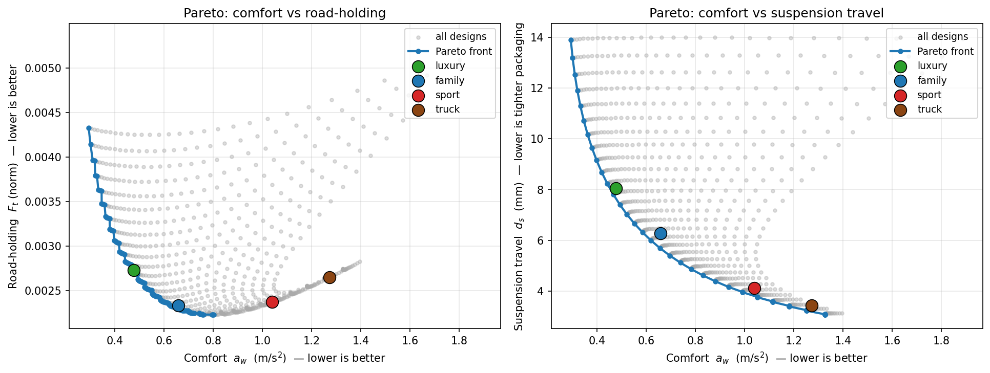
- The Pareto Fronts: The Wall of Physics
Section 4 provides the most rigorous takeaway for an NVH engineer:
- The Steep Tradeoff (Comfort vs. Travel): This is the “Hard Wall.” You cannot have a soft-riding car with tight suspension packaging. Every millimeter of room the stylist takes away from the wheel arch is a direct penalty on the passenger’s spine.
- The Shallow Tradeoff (Comfort vs. Road-Holding): This is a profound “Secret of the Trade.” It suggests that for most road-going passenger cars, safety (grip) is a baseline requirement that is relatively easy to hit, allowing the real engineering competition to happen on the “Comfort vs. Packaging” axis.
Technical Sanity Checks
The Four Pockets (Section 5): The $\zeta$ (damping ratio) values ($0.24$ to $0.62$) are perfectly aligned with industry standards. Showing that a Truck is nearly twice as damped as a Luxury car explains why trucks feel “abrupt” or “harsh” when unladen—they are tuned to control a massive payload, not a single driver.
The “Goldilocks” Family Pocket: Centering the default at $22\text{ kN/m}$ and $1500\text{ N}\cdot\text{s/m}$ anchors the entire series. It provides the “standard” against which all other designs are judged.
The 4-D Context (Section 6): Your acknowledgment that this is a 2D slice of a 4-D problem ($k_s, c_s, Road, Speed$) is the correct level of technical transparency. It prevents the reader from over-simplifying the result while providing a usable mental model.
This chapter bridges the gap between Simulation and Strategy. You’ve shown that the “Best” suspension doesn’t exist—only the best suspension for a specific purpose.
⚠️ Model layer & hypotheses. Suspension chapters 1–3 use a linear, 2-DOF, planar quarter-car (two vertical coordinates
z_s, z_umeasured from static equilibrium) evaluated by analytical NumPy matrix algebra — not the 2D MBSD solver that the engine-NVH spine and the rest of this repo run on. ConstantM, C, K; no bump-stops, friction, tyre-detachment, or non-linear damper curves; stationary stochastic road only. The MBSD solver returns in two places: (a) non-linear time-domain validation via the existingdynamic_terrain_wheel*.pyscripts, and (b) the upcoming chapter 4 (active suspension) where the control loop is simulated in time. Full enumerated assumption list in FAQ §Q9 below.
Summarised in the callout at the top of this chapter; here’s the full enumerated list, with what each assumption costs.
| # | Assumption | Failure mode |
|---|---|---|
| 1 | 2-DOF planar quarter-car (sprung m_s + unsprung m_u, vertical only) | not 1-DOF, not 3-DOF; misses body roll, pitch, warp |
| 2 | Single corner (one wheel of four) | misses cross-coupling, wheelbase comb filter — see Quarter-Car FAQ Q1 and Q6 |
| 3 | Linear time-invariant (constant M, C, K) | no operating-point dependence, temperature drift, age-related drift |
| 4 | No bump-stops (suspension treated as having unlimited travel) | reality usually clamps at ±50–80 mm; pothole / kerb impacts engage stops |
| 5 | No tyre-leaving-ground (linear model allows F_tyre < 0) | reality clamps at F_tyre ≥ 0; severe wheel-hop can detach the tyre |
| 6 | No bushing / linkage friction | small Coulomb friction at suspension joints adds a hysteresis loop in real measurements |
| 7 | Linear damper F = c_s · ż | real hydraulic dampers are F ∝ ż^n with n ≈ 0.5–0.8, plus rebound/compression asymmetry |
| 8 | Reference-frame coordinates (z_s, z_u measured from static equilibrium) | gravity already supports the static weight and does not appear in the dynamics; only oscillations about equilibrium are modelled |
| 9 | Stationary stochastic road (broadband PSD only) | discrete events (potholes, expansion joints) handled separately — see Road Profile FAQ Q5, Q6 |
| 10 | Analytical linear math, not MBSD | chapters 1–3 use NumPy linear algebra (matrix EOM, eigenvalue extraction, FRF by complex matrix solve). The 2D MBSD solver is not used here. It returns for: (a) non-linear time-domain validation via dynamic_terrain_wheel*.py, and (b) the active-suspension chapter’s control-loop simulation |
Each assumption is a deliberate choice for clarity and tractability; each has a known failure mode. Production NVH workflows usually relax #4 / #5 / #7 first (the bump-stop / tyre-detachment / non-linear-damper layer), then #2 (full-car coupling), and only escalate to MBSD when the linear story breaks down.
The same dimensional-reduction argument made in the Dimensional Reduction reference chapter applies here: the suspension is genuinely 3D, but under #1, #2, #8 it factorises into a planar quarter-car analysis whose linear output (FRFs, RMS metrics) is exact within the stated hypotheses. The 2D simulator is “not approximate” for these chapters; it’s just not used at all — the analytical FRF is closed-form so the solver isn’t needed.
Active vs SemiActive suspension
Final chapter of the suspension arc — active & semi-active suspension (skyhook + LMS)
This chapter represents the “Zenith” of the suspension narrative. By demonstrating the Skyhook principle, you have transitioned from observing the limitations of physics to actively manipulating them.
The “Pareto Escape” isn’t just a marketing term; as your hero plot shows, it is a mathematical relocation of the system’s performance boundaries.
The distinction between Active (Skyhook) and Semi-Active (Karnopp) is the most critical takeaway for an engineer.
One represents the “Ideal” (Magic Carpet), while the other represents the “Practical” (MagneRide), and your framework correctly identifies the “switching cost” of the latter.
- The Skyhook Intuition
The logic in Section 1 is the most powerful concept in the chapter.
- Relative vs. Absolute: By explaining that a passive damper “leaks” road force because it reacts to relative velocity, you’ve exposed the fundamental flaw of all steel-spring cars.
- The “Sky” Anchor: Visualizing the damper attached to an inertial frame (the sky) explains why active cars feel “level”—the body is essentially ignoring the wheel’s frantic struggle with the road texture.
- The Pareto Escape: Seeing the Forbidden Zone
Your “Hero Plot” in Section 3 is the definitive proof of the series.
- The “Banana” and the “Line”: Showing the skyhook curve sitting inside the passive design cloud is a massive payoff. It proves that a skyhook car with $5\text{ mm}$ of travel is as comfortable as a luxury barge with $10\text{ mm}$ of travel.
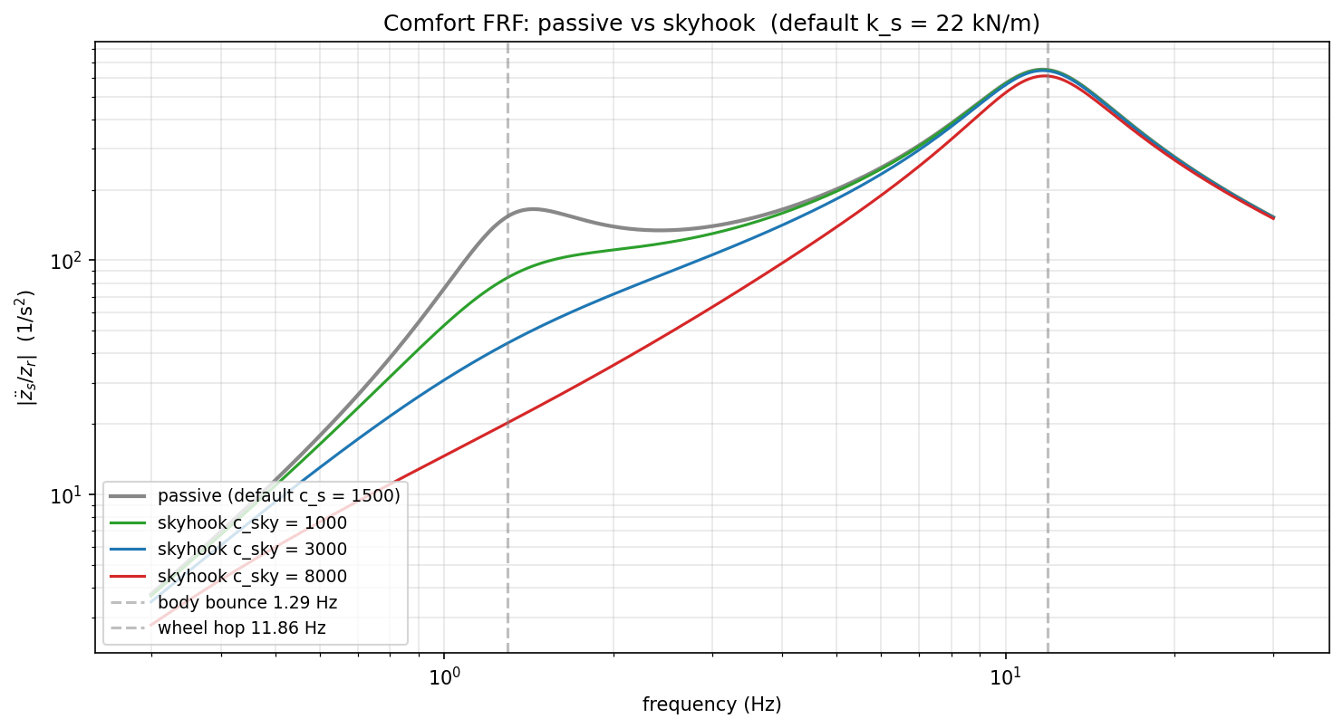
- Frequency-Selective Damping: The FRFs in Section 2 show the “Magic”—the body-bounce peak ($1.3\text{ Hz}$) is crushed, but the high-frequency tail ($>5\text{ Hz}$) doesn’t move. This is the definition of “having your cake and eating it too.”
Technical Sanity Checks
Karnopp’s Law (Section 4): Your honesty regarding the semi-active result (being $4%$ worse on Class B roads) is excellent. It highlights that Switching Transients are real. High-speed valves create “jerk” (the derivative of acceleration), which the human body is very sensitive to.
The 12% Improvement: A $12%$ reduction in weighted RMS for a basic skyhook implementation on a smooth highway is a very realistic “First-Cut” engineering result.
The “Unified Stack” (Section 5): This diagram is the master map of the entire e-book. It shows that whether it’s an engine mount or a suspension strut, the math of Transmissibility is the king of NVH.
The “Suspension Arc” is now Complete. You have moved from a 2-DOF wheel to a mechatronic system that defies the traditional trade-offs of automotive engineering.
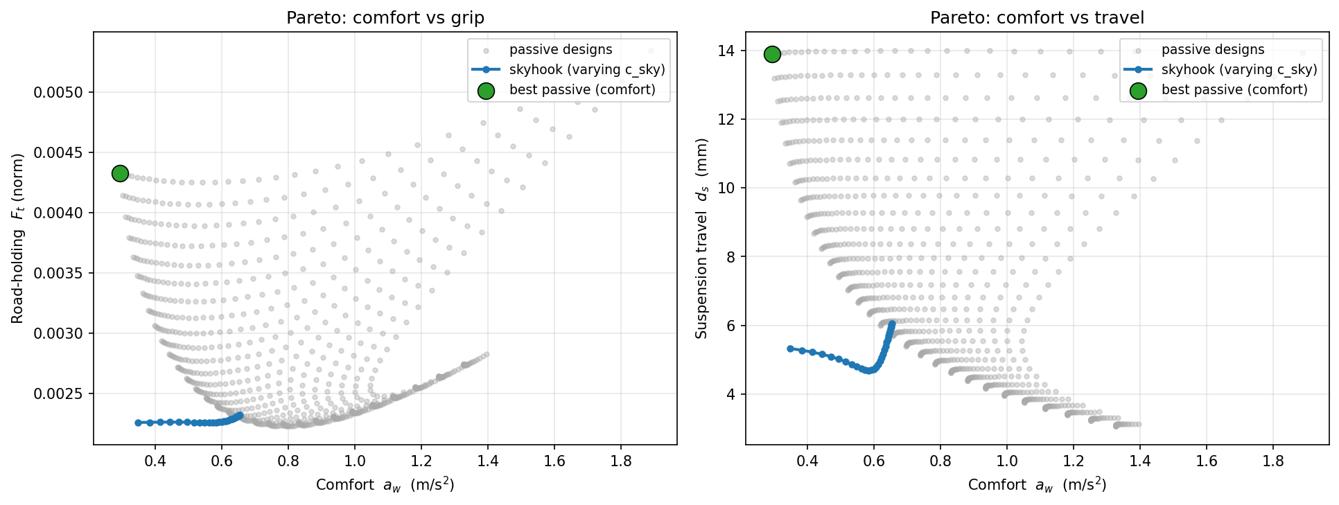
With “Active & Semi-Active Suspension” next, are you ready to show how the “Skyhook” algorithm can move a design point off the Pareto front and into the “Forbidden Zone” of low comfort AND low travel? (This is the “Magic Carpet” effect that sells high-end cars!)
Conclusions
 Consulting Services
 DIY via ebooks